

7.3 Theory for Remodeling in 1D
349
With t treated as a constant, evaluating the integral gives
t
0
e
−k n − (t−τ ) dτ = e
−k n − t
t
0
e
k n − τ dτ =
e −k n − t
k n −
e
k n − t
− 1
=
1
k n −
1 − e
−k n − t
.
Substituting this result into (7.14) gives
J
n (t) = J
n
0
e
−k n − t
+
k n +
k n −
1 − e
−k n − t
.
(7.15)
Results
Results are shown for J n
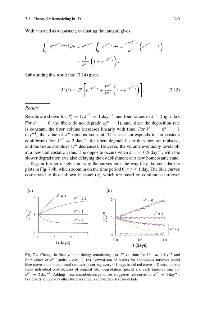
0 = 1, k n + = 1 day −1 , and four values of k n − (Fig. 7.4a).
For k n − = 0, the fibers do not degrade (q n = 1), and, since the deposition rate
is constant, the fiber volume increases linearly with time. For k n − = k n + = 1
day −1 , the value of J n remains constant. This case corresponds to homeostatic
equilibrium. For k n − = 2 day −1 , the fibers degrade faster than they are replaced,
and the tissue atrophies (J n decreases). However, the volume eventually levels off
at a new homeostatic value. The opposite occurs when k n − = 0.5 day −1 , with the
slower degradation rate also delaying the establishment of a new homeostatic state.
To gain further insight into why the curves look the way they do, consider the
plots in Fig. 7.4b, which zoom in on the time period 0 ≤ t ≤ 1 day. The blue curves
correspond to those shown in panel (a), which are based on continuous turnover
Fig. 7.4 Change in fiber volume during remodeling. (a) J n vs. time for k n + = 1 day −1 and
four values of k n − (units = day −1 ). (b) Comparison of results for continuous turnover (solid
blue curves) and incremental turnover occurring every 0.1 days (solid red curves). Dashed curves
show individual contributions of original fiber degradation (green) and each turnover time for
k n − = 2 day −1 . Adding these contributions produces staggered red curve for k n − = 2 day −1 .
For clarity, only every other turnover time is shown. See text for details
349
With t treated as a constant, evaluating the integral gives
t
0
e
−k n − (t−τ ) dτ = e
−k n − t
t
0
e
k n − τ dτ =
e −k n − t
k n −
e
k n − t
− 1
=
1
k n −
1 − e
−k n − t
.
Substituting this result into (7.14) gives
J
n (t) = J
n
0
e
−k n − t
+
k n +
k n −
1 − e
−k n − t
.
(7.15)
Results
Results are shown for J n
0 = 1, k n + = 1 day −1 , and four values of k n − (Fig. 7.4a).
For k n − = 0, the fibers do not degrade (q n = 1), and, since the deposition rate
is constant, the fiber volume increases linearly with time. For k n − = k n + = 1
day −1 , the value of J n remains constant. This case corresponds to homeostatic
equilibrium. For k n − = 2 day −1 , the fibers degrade faster than they are replaced,
and the tissue atrophies (J n decreases). However, the volume eventually levels off
at a new homeostatic value. The opposite occurs when k n − = 0.5 day −1 , with the
slower degradation rate also delaying the establishment of a new homeostatic state.
To gain further insight into why the curves look the way they do, consider the
plots in Fig. 7.4b, which zoom in on the time period 0 ≤ t ≤ 1 day. The blue curves
correspond to those shown in panel (a), which are based on continuous turnover
Fig. 7.4 Change in fiber volume during remodeling. (a) J n vs. time for k n + = 1 day −1 and
four values of k n − (units = day −1 ). (b) Comparison of results for continuous turnover (solid
blue curves) and incremental turnover occurring every 0.1 days (solid red curves). Dashed curves
show individual contributions of original fiber degradation (green) and each turnover time for
k n − = 2 day −1 . Adding these contributions produces staggered red curve for k n − = 2 day −1 .
For clarity, only every other turnover time is shown. See text for details