

6.11 Case Study: Functional Adaptation in Arteries
325
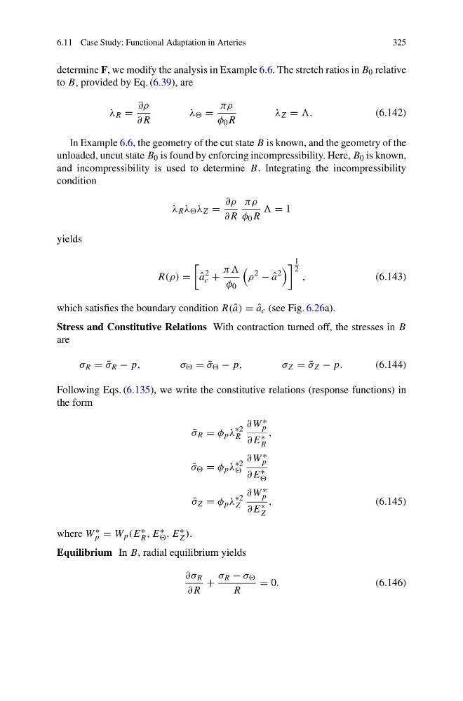
determine F, we modify the analysis in Example 6.6. The stretch ratios in B 0 relative
to B, provided by Eq. (6.39), are
λ R =
∂ρ
∂R
λ =
πρ
φ 0 R
λ Z = .
(6.142)
In Example 6.6, the geometry of the cut state B is known, and the geometry of the
unloaded, uncut state B 0 is found by enforcing incompressibility. Here, B 0 is known,
and incompressibility is used to determine B. Integrating the incompressibility
condition
λ R λ λ Z =
∂ρ
∂R
πρ
φ 0 R
= 1
yields
R(ρ) =
ˆ
a
2
c +
ππ
φ 0
ρ
2
− ˆ
a
2
1
2
,
(6.143)
which satisfies the boundary condition R( ˆ
a) = ˆ
a c (see Fig. 6.26a).
Stress and Constitutive Relations With contraction turned off, the stresses in B
are
σ R = ¯
σ R − p,
σ = ¯
σ − p,
σ Z = ¯
σ Z − p.
(6.144)
Following Eqs. (6.135), we write the constitutive relations (response functions) in
the form
¯
σ R = φ p λ
∗2
R
∂W ∗
p
∂E ∗
R
,
¯
σ = φ p λ
∗2
∂W ∗
p
∂E ∗
¯
σ Z = φ p λ
∗2
Z
∂W ∗
p
∂E ∗
Z
,
(6.145)
where W ∗
p = W p (E ∗
R , E ∗
, E ∗
Z ).
Equilibrium In B, radial equilibrium yields
∂σ R
∂R
+
σ R − σ
R
= 0.
(6.146)
325
determine F, we modify the analysis in Example 6.6. The stretch ratios in B 0 relative
to B, provided by Eq. (6.39), are
λ R =
∂ρ
∂R
λ =
πρ
φ 0 R
λ Z = .
(6.142)
In Example 6.6, the geometry of the cut state B is known, and the geometry of the
unloaded, uncut state B 0 is found by enforcing incompressibility. Here, B 0 is known,
and incompressibility is used to determine B. Integrating the incompressibility
condition
λ R λ λ Z =
∂ρ
∂R
πρ
φ 0 R
= 1
yields
R(ρ) =
ˆ
a
2
c +
ππ
φ 0
ρ
2
− ˆ
a
2
1
2
,
(6.143)
which satisfies the boundary condition R( ˆ
a) = ˆ
a c (see Fig. 6.26a).
Stress and Constitutive Relations With contraction turned off, the stresses in B
are
σ R = ¯
σ R − p,
σ = ¯
σ − p,
σ Z = ¯
σ Z − p.
(6.144)
Following Eqs. (6.135), we write the constitutive relations (response functions) in
the form
¯
σ R = φ p λ
∗2
R
∂W ∗
p
∂E ∗
R
,
¯
σ = φ p λ
∗2
∂W ∗
p
∂E ∗
¯
σ Z = φ p λ
∗2
Z
∂W ∗
p
∂E ∗
Z
,
(6.145)
where W ∗
p = W p (E ∗
R , E ∗
, E ∗
Z ).
Equilibrium In B, radial equilibrium yields
∂σ R
∂R
+
σ R − σ
R
= 0.
(6.146)