

296
6 Growth
equation for the function r(R). For some forms of W , an analytical solution could
be found using some mathematical trickery (Chung et al. 1986), but here we follow
an easier route using finite elements, with the strain-energy density function taken
in the form
W = c
I 1 − 3 +
1 − 2ν
ν
J
−2ν/(1−2ν)
− 1
,
(6.84)
as provided by Eq. (3.222) with α = 1 and I 3 = J 2 . Here, ν represents Poisson’s
ratio in the limit of small strain. For ν → 0.5, this expression approaches the
incompressible relation given by Eq. (6.77).
6.8.3 Illustrative Results
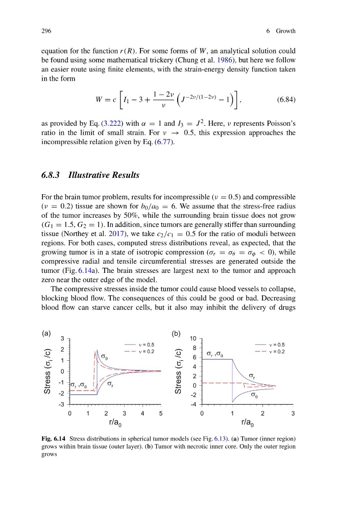
For the brain tumor problem, results for incompressible (ν = 0.5) and compressible
(ν = 0.2) tissue are shown for b 0 /a 0 = 6. We assume that the stress-free radius
of the tumor increases by 50%, while the surrounding brain tissue does not grow
(G 1 = 1.5, G 2 = 1). In addition, since tumors are generally stiffer than surrounding
tissue (Northey et al. 2017), we take c 2 /c 1 = 0.5 for the ratio of moduli between
regions. For both cases, computed stress distributions reveal, as expected, that the
growing tumor is in a state of isotropic compression (σ r = σ θ = σ φ < 0), while
compressive radial and tensile circumferential stresses are generated outside the
tumor (Fig. 6.14a). The brain stresses are largest next to the tumor and approach
zero near the outer edge of the model.
The compressive stresses inside the tumor could cause blood vessels to collapse,
blocking blood flow. The consequences of this could be good or bad. Decreasing
blood flow can starve cancer cells, but it also may inhibit the delivery of drugs
Fig. 6.14 Stress distributions in spherical tumor models (see Fig. 6.13). (a) Tumor (inner region)
grows within brain tissue (outer layer). (b) Tumor with necrotic inner core. Only the outer region
grows
6 Growth
equation for the function r(R). For some forms of W , an analytical solution could
be found using some mathematical trickery (Chung et al. 1986), but here we follow
an easier route using finite elements, with the strain-energy density function taken
in the form
W = c
I 1 − 3 +
1 − 2ν
ν
J
−2ν/(1−2ν)
− 1
,
(6.84)
as provided by Eq. (3.222) with α = 1 and I 3 = J 2 . Here, ν represents Poisson’s
ratio in the limit of small strain. For ν → 0.5, this expression approaches the
incompressible relation given by Eq. (6.77).
6.8.3 Illustrative Results
For the brain tumor problem, results for incompressible (ν = 0.5) and compressible
(ν = 0.2) tissue are shown for b 0 /a 0 = 6. We assume that the stress-free radius
of the tumor increases by 50%, while the surrounding brain tissue does not grow
(G 1 = 1.5, G 2 = 1). In addition, since tumors are generally stiffer than surrounding
tissue (Northey et al. 2017), we take c 2 /c 1 = 0.5 for the ratio of moduli between
regions. For both cases, computed stress distributions reveal, as expected, that the
growing tumor is in a state of isotropic compression (σ r = σ θ = σ φ < 0), while
compressive radial and tensile circumferential stresses are generated outside the
tumor (Fig. 6.14a). The brain stresses are largest next to the tumor and approach
zero near the outer edge of the model.
The compressive stresses inside the tumor could cause blood vessels to collapse,
blocking blood flow. The consequences of this could be good or bad. Decreasing
blood flow can starve cancer cells, but it also may inhibit the delivery of drugs
Fig. 6.14 Stress distributions in spherical tumor models (see Fig. 6.13). (a) Tumor (inner region)
grows within brain tissue (outer layer). (b) Tumor with necrotic inner core. Only the outer region
grows