

4.1 Uniaxial Extension of a Bar
159
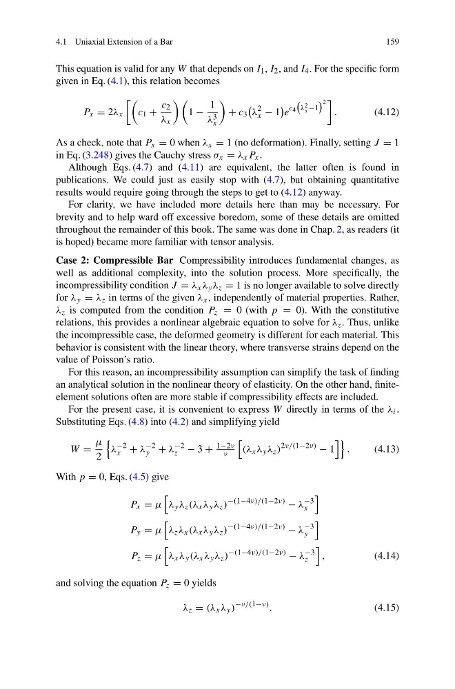
This equation is valid for any W that depends on I 1 , I 2 , and I 4 . For the specific form
given in Eq. (4.1), this relation becomes
P x = 2λ x
c 1 +
c 2
λ x
1 −
1
λ 3
x
+ c 3
λ
2
x − 1
e
c 4
λ 2
x −1
2
.
(4.12)
As a check, note that P x = 0 when λ x = 1 (no deformation). Finally, setting J = 1
in Eq. (3.248) gives the Cauchy stress σ x = λ x P x .
Although Eqs. (4.7) and (4.11) are equivalent, the latter often is found in
publications. We could just as easily stop with (4.7), but obtaining quantitative
results would require going through the steps to get to (4.12) anyway.
For clarity, we have included more details here than may be necessary. For
brevity and to help ward off excessive boredom, some of these details are omitted
throughout the remainder of this book. The same was done in Chap. 2, as readers (it
is hoped) became more familiar with tensor analysis.
Case 2: Compressible Bar Compressibility introduces fundamental changes, as
well as additional complexity, into the solution process. More specifically, the
incompressibility condition J = λ x λ y λ z = 1 is no longer available to solve directly
for λ y = λ z in terms of the given λ x , independently of material properties. Rather,
λ z is computed from the condition P z = 0 (with p = 0). With the constitutive
relations, this provides a nonlinear algebraic equation to solve for λ z . Thus, unlike
the incompressible case, the deformed geometry is different for each material. This
behavior is consistent with the linear theory, where transverse strains depend on the
value of Poisson’s ratio.
For this reason, an incompressibility assumption can simplify the task of finding
an analytical solution in the nonlinear theory of elasticity. On the other hand, finiteelement solutions often are more stable if compressibility effects are included.
For the present case, it is convenient to express W directly in terms of the λ i .
Substituting Eqs. (4.8) into (4.2) and simplifying yield
W =
μ
2
λ
−2
x + λ
−2
y + λ
−2
z − 3 +
1−2ν
ν
(λ x λ y λ z )
2ν/(1−2ν)
− 1
.
(4.13)
With p = 0, Eqs. (4.5) give
P x = μ
λ y λ z (λ x λ y λ z )
−(1−4ν)/(1−2ν)
− λ
−3
x
P y = μ
λ z λ x (λ x λ y λ z )
−(1−4ν)/(1−2ν)
− λ
−3
y
P z = μ
λ x λ y (λ x λ y λ z )
−(1−4ν)/(1−2ν)
− λ
−3
z
,
(4.14)
and solving the equation P z = 0 yields
λ z = (λ x λ y )
−ν/(1−ν) .
(4.15)
159
This equation is valid for any W that depends on I 1 , I 2 , and I 4 . For the specific form
given in Eq. (4.1), this relation becomes
P x = 2λ x
c 1 +
c 2
λ x
1 −
1
λ 3
x
+ c 3
λ
2
x − 1
e
c 4
λ 2
x −1
2
.
(4.12)
As a check, note that P x = 0 when λ x = 1 (no deformation). Finally, setting J = 1
in Eq. (3.248) gives the Cauchy stress σ x = λ x P x .
Although Eqs. (4.7) and (4.11) are equivalent, the latter often is found in
publications. We could just as easily stop with (4.7), but obtaining quantitative
results would require going through the steps to get to (4.12) anyway.
For clarity, we have included more details here than may be necessary. For
brevity and to help ward off excessive boredom, some of these details are omitted
throughout the remainder of this book. The same was done in Chap. 2, as readers (it
is hoped) became more familiar with tensor analysis.
Case 2: Compressible Bar Compressibility introduces fundamental changes, as
well as additional complexity, into the solution process. More specifically, the
incompressibility condition J = λ x λ y λ z = 1 is no longer available to solve directly
for λ y = λ z in terms of the given λ x , independently of material properties. Rather,
λ z is computed from the condition P z = 0 (with p = 0). With the constitutive
relations, this provides a nonlinear algebraic equation to solve for λ z . Thus, unlike
the incompressible case, the deformed geometry is different for each material. This
behavior is consistent with the linear theory, where transverse strains depend on the
value of Poisson’s ratio.
For this reason, an incompressibility assumption can simplify the task of finding
an analytical solution in the nonlinear theory of elasticity. On the other hand, finiteelement solutions often are more stable if compressibility effects are included.
For the present case, it is convenient to express W directly in terms of the λ i .
Substituting Eqs. (4.8) into (4.2) and simplifying yield
W =
μ
2
λ
−2
x + λ
−2
y + λ
−2
z − 3 +
1−2ν
ν
(λ x λ y λ z )
2ν/(1−2ν)
− 1
.
(4.13)
With p = 0, Eqs. (4.5) give
P x = μ
λ y λ z (λ x λ y λ z )
−(1−4ν)/(1−2ν)
− λ
−3
x
P y = μ
λ z λ x (λ x λ y λ z )
−(1−4ν)/(1−2ν)
− λ
−3
y
P z = μ
λ x λ y (λ x λ y λ z )
−(1−4ν)/(1−2ν)
− λ
−3
z
,
(4.14)
and solving the equation P z = 0 yields
λ z = (λ x λ y )
−ν/(1−ν) .
(4.15)