

3.4 Analysis of Stress
103
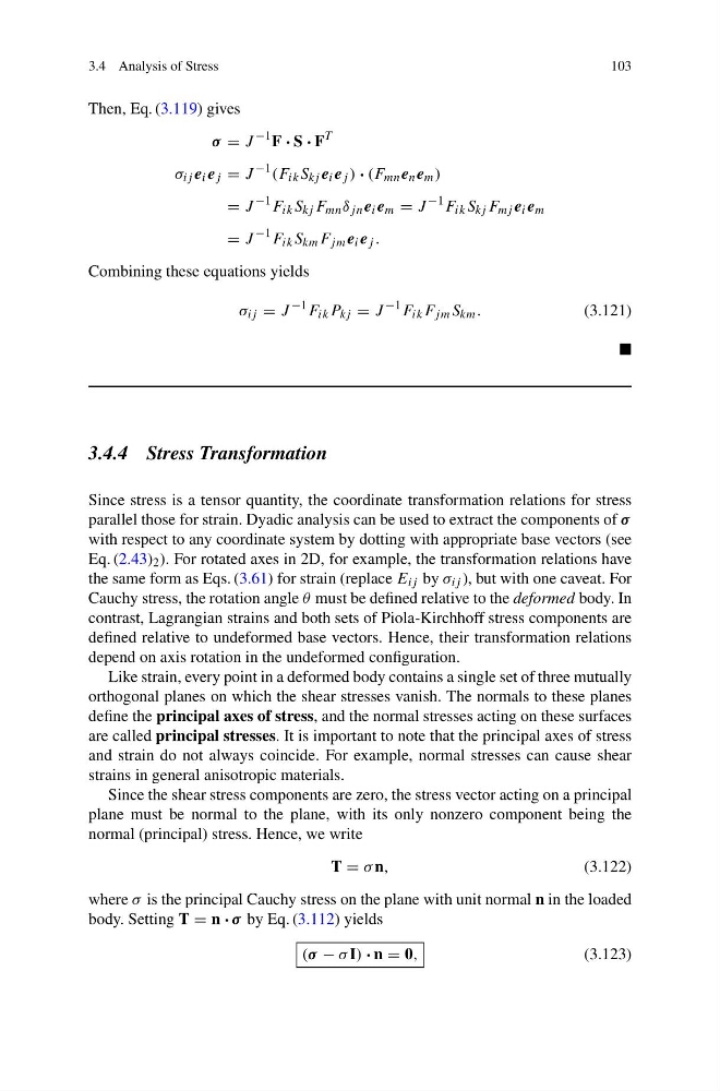
Then, Eq. (3.119) gives
σ = J
−1 F · S · F
T
σ ij e i e j = J
−1 (F ik S kj e i e j ) · (F mn e n e m )
= J
−1 F ik S kj F mn δ jn e i e m = J
−1 F ik S kj F mj e i e m
= J
−1 F ik S km F jm e i e j .
Combining these equations yields
σ ij = J
−1 F ik P kj = J
−1 F ik F jm S km .
(3.121)
3.4.4 Stress Transformation
Since stress is a tensor quantity, the coordinate transformation relations for stress
parallel those for strain. Dyadic analysis can be used to extract the components of σ
with respect to any coordinate system by dotting with appropriate base vectors (see
Eq. (2.43) 2 ). For rotated axes in 2D, for example, the transformation relations have
the same form as Eqs. (3.61) for strain (replace E ij by σ ij ), but with one caveat. For
Cauchy stress, the rotation angle θ must be defined relative to the deformed body. In
contrast, Lagrangian strains and both sets of Piola-Kirchhoff stress components are
defined relative to undeformed base vectors. Hence, their transformation relations
depend on axis rotation in the undeformed configuration.
Like strain, every point in a deformed body contains a single set of three mutually
orthogonal planes on which the shear stresses vanish. The normals to these planes
define the principal axes of stress, and the normal stresses acting on these surfaces
are called principal stresses. It is important to note that the principal axes of stress
and strain do not always coincide. For example, normal stresses can cause shear
strains in general anisotropic materials.
Since the shear stress components are zero, the stress vector acting on a principal
plane must be normal to the plane, with its only nonzero component being the
normal (principal) stress. Hence, we write
T = σ n,
(3.122)
where σ is the principal Cauchy stress on the plane with unit normal n in the loaded
body. Setting T = n · σ by Eq. (3.112) yields
(σ − σ I) · n = 0,
(3.123)
103
Then, Eq. (3.119) gives
σ = J
−1 F · S · F
T
σ ij e i e j = J
−1 (F ik S kj e i e j ) · (F mn e n e m )
= J
−1 F ik S kj F mn δ jn e i e m = J
−1 F ik S kj F mj e i e m
= J
−1 F ik S km F jm e i e j .
Combining these equations yields
σ ij = J
−1 F ik P kj = J
−1 F ik F jm S km .
(3.121)
3.4.4 Stress Transformation
Since stress is a tensor quantity, the coordinate transformation relations for stress
parallel those for strain. Dyadic analysis can be used to extract the components of σ
with respect to any coordinate system by dotting with appropriate base vectors (see
Eq. (2.43) 2 ). For rotated axes in 2D, for example, the transformation relations have
the same form as Eqs. (3.61) for strain (replace E ij by σ ij ), but with one caveat. For
Cauchy stress, the rotation angle θ must be defined relative to the deformed body. In
contrast, Lagrangian strains and both sets of Piola-Kirchhoff stress components are
defined relative to undeformed base vectors. Hence, their transformation relations
depend on axis rotation in the undeformed configuration.
Like strain, every point in a deformed body contains a single set of three mutually
orthogonal planes on which the shear stresses vanish. The normals to these planes
define the principal axes of stress, and the normal stresses acting on these surfaces
are called principal stresses. It is important to note that the principal axes of stress
and strain do not always coincide. For example, normal stresses can cause shear
strains in general anisotropic materials.
Since the shear stress components are zero, the stress vector acting on a principal
plane must be normal to the plane, with its only nonzero component being the
normal (principal) stress. Hence, we write
T = σ n,
(3.122)
where σ is the principal Cauchy stress on the plane with unit normal n in the loaded
body. Setting T = n · σ by Eq. (3.112) yields
(σ − σ I) · n = 0,
(3.123)