

64
P. Liu
where C μ is an empirical constant. Turbulent kinetic energy K and turbulent energy dissipation rate ε are closed by the transport equation. For the
standard K – ε turbulence model,
The turbulent kinetic energy K equation is
∂ K
∂t
+ u j
∂ K
∂ x j
=
∂
∂ x j
ν t
σ K
+ ν
∂ K
∂ x j
+ P − ε
The turbulent kinetic energy dissipation rate equation ε is
∂ε
∂t
+ u j
∂ε
∂ x j
=
∂
∂ x j
ν t
σ ε
+ ν
∂ε
∂ x j
+ C ε1
ε
K
P − C ε 2
ε 2
K
where P = −u
i u
j
∂u i
∂ x j
is the turbulent kinetic energy generation term. The
empirical constants in the model should be determined by experiments. At
present, most scholars recommend the values of the constants as follows: C μ
= 0.07 ~ 0.09, σ K = 1.0, σ ε = 1.3, C ε1 = 1.41~1.45, C ε2 = 1.9~1.92.
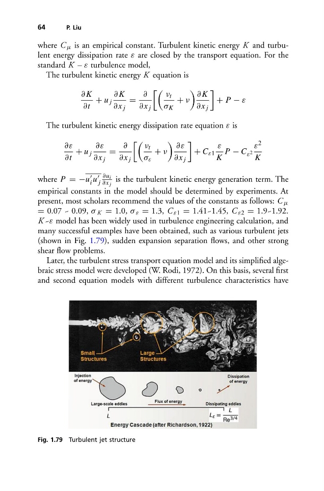
K ~ε model has been widely used in turbulence engineering calculation, and
many successful examples have been obtained, such as various turbulent jets
(shown in Fig. 1.79), sudden expansion separation flows, and other strong
shear flow problems.
Later, the turbulent stress transport equation model and its simplified algebraic stress model were developed (W. Rodi, 1972). On this basis, several first
and second equation models with different turbulence characteristics have
Fig. 1.79 Turbulent jet structure
P. Liu
where C μ is an empirical constant. Turbulent kinetic energy K and turbulent energy dissipation rate ε are closed by the transport equation. For the
standard K – ε turbulence model,
The turbulent kinetic energy K equation is
∂ K
∂t
+ u j
∂ K
∂ x j
=
∂
∂ x j
ν t
σ K
+ ν
∂ K
∂ x j
+ P − ε
The turbulent kinetic energy dissipation rate equation ε is
∂ε
∂t
+ u j
∂ε
∂ x j
=
∂
∂ x j
ν t
σ ε
+ ν
∂ε
∂ x j
+ C ε1
ε
K
P − C ε 2
ε 2
K
where P = −u
i u
j
∂u i
∂ x j
is the turbulent kinetic energy generation term. The
empirical constants in the model should be determined by experiments. At
present, most scholars recommend the values of the constants as follows: C μ
= 0.07 ~ 0.09, σ K = 1.0, σ ε = 1.3, C ε1 = 1.41~1.45, C ε2 = 1.9~1.92.
K ~ε model has been widely used in turbulence engineering calculation, and
many successful examples have been obtained, such as various turbulent jets
(shown in Fig. 1.79), sudden expansion separation flows, and other strong
shear flow problems.
Later, the turbulent stress transport equation model and its simplified algebraic stress model were developed (W. Rodi, 1972). On this basis, several first
and second equation models with different turbulence characteristics have
Fig. 1.79 Turbulent jet structure