

4 Computational Fluid Dynamics
305
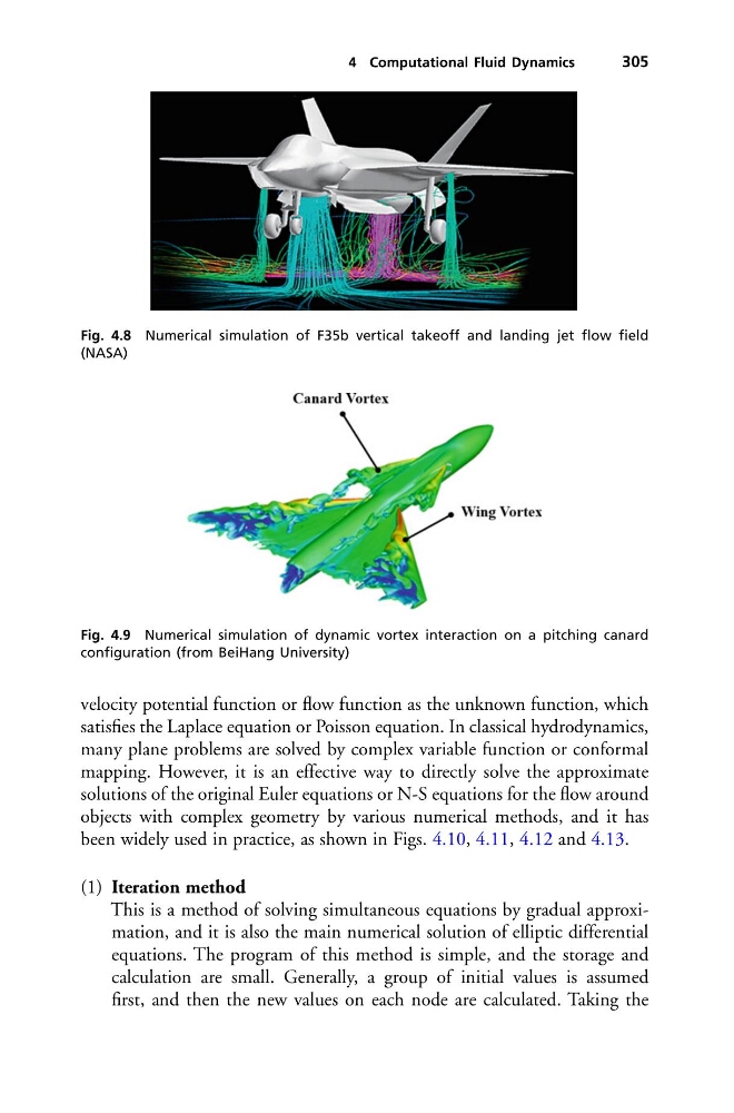
Fig. 4.8 Numerical simulation of F35b vertical takeoff and landing jet flow field
(NASA)
Fig. 4.9 Numerical simulation of dynamic vortex interaction on a pitching canard
configuration (from BeiHang University)
velocity potential function or flow function as the unknown function, which
satisfies the Laplace equation or Poisson equation. In classical hydrodynamics,
many plane problems are solved by complex variable function or conformal
mapping. However, it is an effective way to directly solve the approximate
solutions of the original Euler equations or N-S equations for the flow around
objects with complex geometry by various numerical methods, and it has
been widely used in practice, as shown in Figs. 4.10, 4.11, 4.12 and 4.13.
(1) Iteration method
This is a method of solving simultaneous equations by gradual approximation, and it is also the main numerical solution of elliptic differential
equations. The program of this method is simple, and the storage and
calculation are small. Generally, a group of initial values is assumed
first, and then the new values on each node are calculated. Taking the
305
Fig. 4.8 Numerical simulation of F35b vertical takeoff and landing jet flow field
(NASA)
Fig. 4.9 Numerical simulation of dynamic vortex interaction on a pitching canard
configuration (from BeiHang University)
velocity potential function or flow function as the unknown function, which
satisfies the Laplace equation or Poisson equation. In classical hydrodynamics,
many plane problems are solved by complex variable function or conformal
mapping. However, it is an effective way to directly solve the approximate
solutions of the original Euler equations or N-S equations for the flow around
objects with complex geometry by various numerical methods, and it has
been widely used in practice, as shown in Figs. 4.10, 4.11, 4.12 and 4.13.
(1) Iteration method
This is a method of solving simultaneous equations by gradual approximation, and it is also the main numerical solution of elliptic differential
equations. The program of this method is simple, and the storage and
calculation are small. Generally, a group of initial values is assumed
first, and then the new values on each node are calculated. Taking the