

lower support with a displacement, u s (Fig. 9.6b).
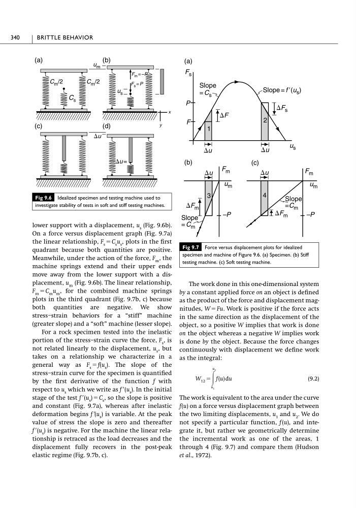
On a force versus displacement graph (Fig. 9.7a)
the linear relationship, F s ϭ C s u s , plots in the first
quadrant because both quantities are positive.
Meanwhile, under the action of the force, F m , the
machine springs extend and their upper ends
move away from the lower support with a displacement, u m (Fig. 9.6b). The linear relationship,
F m ϭ C m u m , for the combined machine springs
plots in the third quadrant (Fig. 9.7b, c) because
both quantities are negative. We show
stress–strain behaviors for a “stiff” machine
(greater slope) and a “soft” machine (lesser slope).
For a rock specimen tested into the inelastic
portion of the stress–strain curve the force, F s , is
not related linearly to the displacement, u s , but
takes on a relationship we characterize in a
general way as F s ϭ f(u s ). The slope of the
stress–strain curve for the specimen is quantified
by the first derivative of the function f with
respect to u s which we write as f Ј(u s ). In the initial
stage of the test f Ј(u s ) ϭ C s , so the slope is positive
and constant (Fig. 9.7a), whereas after inelastic
deformation begins fЈ(u s ) is variable. At the peak
value of stress the slope is zero and thereafter
f Ј(u s ) is negative. For the machine the linear relationship is retraced as the load decreases and the
displacement fully recovers in the post-peak
elastic regime (Fig. 9.7b, c).
The work done in this one-dimensional system
by a constant applied force on an object is defined
as the product of the force and displacement magnitudes, W ϭ Fu. Work is positive if the force acts
in the same direction as the displacement of the
object, so a positive W implies that work is done
on the object whereas a negative W implies work
is done by the object. Because the force changes
continuously with displacement we define work
as the integral:
(9.2)
The work is equivalent to the area under the curve
f(u) on a force versus displacement graph between
the two limiting displacements, u 1 and u 2 . We do
not specify a particular function, f (u), and integrate it, but rather we geometrically determine
the incremental work as one of the areas, 1
through 4 (Fig. 9.7) and compare them (Hudson
et al., 1972).
W 12 ϭ Ύ
u 2
u 1
f (u) du
340
BRITTLE BEHAVIOR
Fig 9.6 Idealized specimen and testing machine used to
investigate stability of tests in soft and stiff testing machines.
(a)
(b)
(c)
(d)
C m /2
C m /2
C s
u m
u s
F m = –P
F s = P
⌬u
⌬u =
x
y
Fig 9.7 Force versus displacement plots for idealized
specimen and machine of Figure 9.6. (a) Specimen. (b) Stiff
testing machine. (c) Soft testing machine.
P
⌬F
⌬F s
⌬u
⌬u
u s
Slope
= C s
Slope = f Ј(u s )
⌬u
F m
Slope
=C m
Slope
= C m
⌬F m
⌬F m
–P
–P
1
2
4
3
F
(b)
(a)
(c)
F s
F m
⌬u
u m
u m
On a force versus displacement graph (Fig. 9.7a)
the linear relationship, F s ϭ C s u s , plots in the first
quadrant because both quantities are positive.
Meanwhile, under the action of the force, F m , the
machine springs extend and their upper ends
move away from the lower support with a displacement, u m (Fig. 9.6b). The linear relationship,
F m ϭ C m u m , for the combined machine springs
plots in the third quadrant (Fig. 9.7b, c) because
both quantities are negative. We show
stress–strain behaviors for a “stiff” machine
(greater slope) and a “soft” machine (lesser slope).
For a rock specimen tested into the inelastic
portion of the stress–strain curve the force, F s , is
not related linearly to the displacement, u s , but
takes on a relationship we characterize in a
general way as F s ϭ f(u s ). The slope of the
stress–strain curve for the specimen is quantified
by the first derivative of the function f with
respect to u s which we write as f Ј(u s ). In the initial
stage of the test f Ј(u s ) ϭ C s , so the slope is positive
and constant (Fig. 9.7a), whereas after inelastic
deformation begins fЈ(u s ) is variable. At the peak
value of stress the slope is zero and thereafter
f Ј(u s ) is negative. For the machine the linear relationship is retraced as the load decreases and the
displacement fully recovers in the post-peak
elastic regime (Fig. 9.7b, c).
The work done in this one-dimensional system
by a constant applied force on an object is defined
as the product of the force and displacement magnitudes, W ϭ Fu. Work is positive if the force acts
in the same direction as the displacement of the
object, so a positive W implies that work is done
on the object whereas a negative W implies work
is done by the object. Because the force changes
continuously with displacement we define work
as the integral:
(9.2)
The work is equivalent to the area under the curve
f(u) on a force versus displacement graph between
the two limiting displacements, u 1 and u 2 . We do
not specify a particular function, f (u), and integrate it, but rather we geometrically determine
the incremental work as one of the areas, 1
through 4 (Fig. 9.7) and compare them (Hudson
et al., 1972).
W 12 ϭ Ύ
u 2
u 1
f (u) du
340
BRITTLE BEHAVIOR
Fig 9.6 Idealized specimen and testing machine used to
investigate stability of tests in soft and stiff testing machines.
(a)
(b)
(c)
(d)
C m /2
C m /2
C s
u m
u s
F m = –P
F s = P
⌬u
⌬u =
x
y
Fig 9.7 Force versus displacement plots for idealized
specimen and machine of Figure 9.6. (a) Specimen. (b) Stiff
testing machine. (c) Soft testing machine.
P
⌬F
⌬F s
⌬u
⌬u
u s
Slope
= C s
Slope = f Ј(u s )
⌬u
F m
Slope
=C m
Slope
= C m
⌬F m
⌬F m
–P
–P
1
2
4
3
F
(b)
(a)
(c)
F s
F m
⌬u
u m
u m