

106
S.O. Adamson et al.
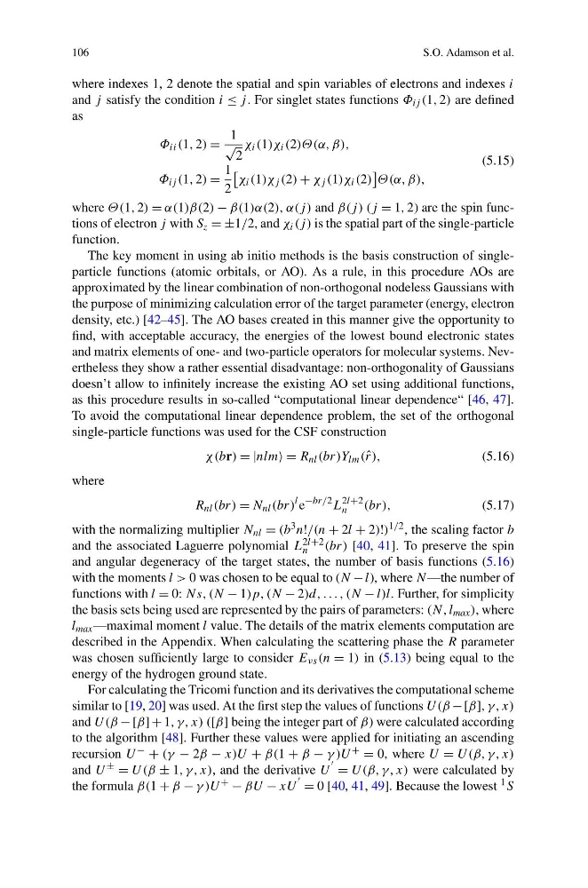
where indexes 1, 2 denote the spatial and spin variables of electrons and indexes i
and j satisfy the condition i ≤ j . For singlet states functions Φ ij (1, 2) are defined
as
Φ ii (1, 2) =
1
√
2
χ i (1)χ i (2)Θ(α, β),
Φ ij (1, 2) =
1
2
χ i (1)χ j (2) + χ j (1)χ i (2)
Θ(α, β),
(5.15)
where Θ(1, 2) = α(1)β(2) − β(1)α(2), α(j ) and β(j ) (j = 1, 2) are the spin functions of electron j with S z = ±1/2, and χ i (j ) is the spatial part of the single-particle
function.
The key moment in using ab initio methods is the basis construction of singleparticle functions (atomic orbitals, or AO). As a rule, in this procedure AOs are
approximated by the linear combination of non-orthogonal nodeless Gaussians with
the purpose of minimizing calculation error of the target parameter (energy, electron
density, etc.) [42–45]. The AO bases created in this manner give the opportunity to
find, with acceptable accuracy, the energies of the lowest bound electronic states
and matrix elements of one- and two-particle operators for molecular systems. Nevertheless they show a rather essential disadvantage: non-orthogonality of Gaussians
doesn’t allow to infinitely increase the existing AO set using additional functions,
as this procedure results in so-called “computational linear dependence“ [46, 47].
To avoid the computational linear dependence problem, the set of the orthogonal
single-particle functions was used for the CSF construction
χ(br) = |nlm = R nl (br)Y lm (ˆ r),
(5.16)
where
R nl (br) = N nl (br)
l e
−br/2 L
2l+2
n
(br),
(5.17)
with the normalizing multiplier N nl = (b 3 n!/(n + 2l + 2)!) 1/2 , the scaling factor b
and the associated Laguerre polynomial L 2l+2
n
(br) [40, 41]. To preserve the spin
and angular degeneracy of the target states, the number of basis functions (5.16)
with the moments l > 0 was chosen to be equal to (N − l), where N —the number of
functions with l = 0: Ns, (N − 1)p, (N − 2)d, . . . , (N − l)l. Further, for simplicity
the basis sets being used are represented by the pairs of parameters: (N, l max ), where
l max —maximal moment l value. The details of the matrix elements computation are
described in the Appendix. When calculating the scattering phase the R parameter
was chosen sufficiently large to consider E νs (n = 1) in (5.13) being equal to the
energy of the hydrogen ground state.
For calculating the Tricomi function and its derivatives the computational scheme
similar to [19, 20] was used. At the first step the values of functions U(β − [β], γ, x)
and U(β − [β] + 1, γ, x) ([β] being the integer part of β) were calculated according
to the algorithm [48]. Further these values were applied for initiating an ascending
recursion U − + (γ − 2β − x)U + β(1 + β − γ )U + = 0, where U = U(β, γ, x)
and U ± = U(β ± 1, γ, x), and the derivative U
= U(β, γ, x) were calculated by
the formula β(1 + β − γ )U + − βU − xU
= 0 [40, 41, 49]. Because the lowest 1 S
S.O. Adamson et al.
where indexes 1, 2 denote the spatial and spin variables of electrons and indexes i
and j satisfy the condition i ≤ j . For singlet states functions Φ ij (1, 2) are defined
as
Φ ii (1, 2) =
1
√
2
χ i (1)χ i (2)Θ(α, β),
Φ ij (1, 2) =
1
2
χ i (1)χ j (2) + χ j (1)χ i (2)
Θ(α, β),
(5.15)
where Θ(1, 2) = α(1)β(2) − β(1)α(2), α(j ) and β(j ) (j = 1, 2) are the spin functions of electron j with S z = ±1/2, and χ i (j ) is the spatial part of the single-particle
function.
The key moment in using ab initio methods is the basis construction of singleparticle functions (atomic orbitals, or AO). As a rule, in this procedure AOs are
approximated by the linear combination of non-orthogonal nodeless Gaussians with
the purpose of minimizing calculation error of the target parameter (energy, electron
density, etc.) [42–45]. The AO bases created in this manner give the opportunity to
find, with acceptable accuracy, the energies of the lowest bound electronic states
and matrix elements of one- and two-particle operators for molecular systems. Nevertheless they show a rather essential disadvantage: non-orthogonality of Gaussians
doesn’t allow to infinitely increase the existing AO set using additional functions,
as this procedure results in so-called “computational linear dependence“ [46, 47].
To avoid the computational linear dependence problem, the set of the orthogonal
single-particle functions was used for the CSF construction
χ(br) = |nlm = R nl (br)Y lm (ˆ r),
(5.16)
where
R nl (br) = N nl (br)
l e
−br/2 L
2l+2
n
(br),
(5.17)
with the normalizing multiplier N nl = (b 3 n!/(n + 2l + 2)!) 1/2 , the scaling factor b
and the associated Laguerre polynomial L 2l+2
n
(br) [40, 41]. To preserve the spin
and angular degeneracy of the target states, the number of basis functions (5.16)
with the moments l > 0 was chosen to be equal to (N − l), where N —the number of
functions with l = 0: Ns, (N − 1)p, (N − 2)d, . . . , (N − l)l. Further, for simplicity
the basis sets being used are represented by the pairs of parameters: (N, l max ), where
l max —maximal moment l value. The details of the matrix elements computation are
described in the Appendix. When calculating the scattering phase the R parameter
was chosen sufficiently large to consider E νs (n = 1) in (5.13) being equal to the
energy of the hydrogen ground state.
For calculating the Tricomi function and its derivatives the computational scheme
similar to [19, 20] was used. At the first step the values of functions U(β − [β], γ, x)
and U(β − [β] + 1, γ, x) ([β] being the integer part of β) were calculated according
to the algorithm [48]. Further these values were applied for initiating an ascending
recursion U − + (γ − 2β − x)U + β(1 + β − γ )U + = 0, where U = U(β, γ, x)
and U ± = U(β ± 1, γ, x), and the derivative U
= U(β, γ, x) were calculated by
the formula β(1 + β − γ )U + − βU − xU
= 0 [40, 41, 49]. Because the lowest 1 S