

104
S.O. Adamson et al.
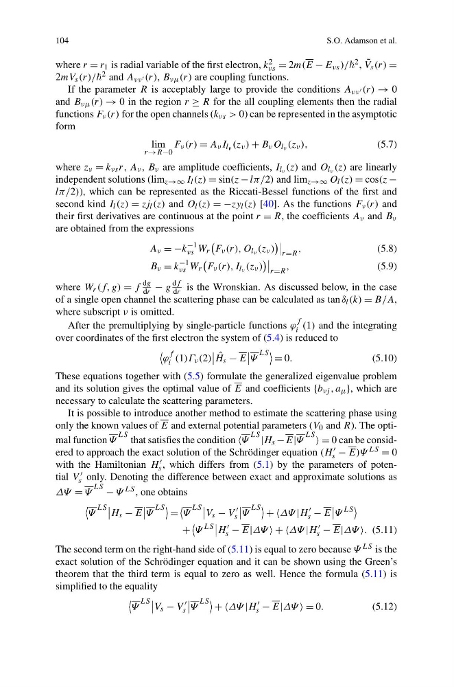
where r = r 1 is radial variable of the first electron, k 2
νs = 2m(E − E νs )/ 2 , ˜
V s (r) =
2mV s (r)/ 2 and A νν (r), B νμ (r) are coupling functions.
If the parameter R is acceptably large to provide the conditions A νν (r) → 0
and B νμ (r) → 0 in the region r ≥ R for the all coupling elements then the radial
functions F ν (r) for the open channels (k νs > 0) can be represented in the asymptotic
form
lim
r→R−0
F ν (r) = A ν I l ν (z ν ) + B ν O l ν (z ν ),
(5.7)
where z ν = k νs r, A ν , B ν are amplitude coefficients, I l ν (z) and O l ν (z) are linearly
independent solutions (lim z→∞ I l (z) = sin(z − lπ/2) and lim z→∞ O l (z) = cos(z −
lπ/2)), which can be represented as the Riccati-Bessel functions of the first and
second kind I l (z) = zj l (z) and O l (z) = −zy l (z) [40]. As the functions F ν (r) and
their first derivatives are continuous at the point r = R, the coefficients A ν and B ν
are obtained from the expressions
A ν = −k
−1
νs W r
F ν (r), O l ν (z ν )
r=R
,
(5.8)
B ν = k
−1
νs W r
F ν (r), I l ν (z ν )
r=R
,
(5.9)
where W r (f, g) = f
dg
dr − g
df
dr is the Wronskian. As discussed below, in the case
of a single open channel the scattering phase can be calculated as tan δ l (k) = B/A,
where subscript ν is omitted.
After the premultiplying by single-particle functions ϕ
f
i (1) and the integrating
over coordinates of the first electron the system of (5.4) is reduced to
ϕ
f
i (1)Γ ν (2)
ˆ
H s − E
Ψ
LS = 0.
(5.10)
These equations together with (5.5) formulate the generalized eigenvalue problem
and its solution gives the optimal value of E and coefficients {b νj , a μ }, which are
necessary to calculate the scattering parameters.
It is possible to introduce another method to estimate the scattering phase using
only the known values of E and external potential parameters (V 0 and R). The optimal function Ψ
LS that satisfies the condition Ψ
LS |H s −E|Ψ
LS = 0 can be considered to approach the exact solution of the Schrödinger equation (H
s − E)Ψ LS = 0
with the Hamiltonian H
s , which differs from (5.1) by the parameters of potential V
s only. Denoting the difference between exact and approximate solutions as
ΔΨ = Ψ
LS − Ψ LS , one obtains
Ψ
LS
H s − E
Ψ
LS =
Ψ
LS
V s − V
s
Ψ
LS + +ΔΨ |H
s − E
Ψ
LS
+
Ψ
LS
H
s − E|ΔΨ + +ΔΨ |H
s − E|ΔΨ . (5.11)
The second term on the right-hand side of (5.11) is equal to zero because Ψ LS is the
exact solution of the Schrödinger equation and it can be shown using the Green’s
theorem that the third term is equal to zero as well. Hence the formula (5.11) is
simplified to the equality
Ψ
LS
V s − V
s
Ψ
LS + +ΔΨ |H
s − E|ΔΨ = 0.
(5.12)
S.O. Adamson et al.
where r = r 1 is radial variable of the first electron, k 2
νs = 2m(E − E νs )/ 2 , ˜
V s (r) =
2mV s (r)/ 2 and A νν (r), B νμ (r) are coupling functions.
If the parameter R is acceptably large to provide the conditions A νν (r) → 0
and B νμ (r) → 0 in the region r ≥ R for the all coupling elements then the radial
functions F ν (r) for the open channels (k νs > 0) can be represented in the asymptotic
form
lim
r→R−0
F ν (r) = A ν I l ν (z ν ) + B ν O l ν (z ν ),
(5.7)
where z ν = k νs r, A ν , B ν are amplitude coefficients, I l ν (z) and O l ν (z) are linearly
independent solutions (lim z→∞ I l (z) = sin(z − lπ/2) and lim z→∞ O l (z) = cos(z −
lπ/2)), which can be represented as the Riccati-Bessel functions of the first and
second kind I l (z) = zj l (z) and O l (z) = −zy l (z) [40]. As the functions F ν (r) and
their first derivatives are continuous at the point r = R, the coefficients A ν and B ν
are obtained from the expressions
A ν = −k
−1
νs W r
F ν (r), O l ν (z ν )
r=R
,
(5.8)
B ν = k
−1
νs W r
F ν (r), I l ν (z ν )
r=R
,
(5.9)
where W r (f, g) = f
dg
dr − g
df
dr is the Wronskian. As discussed below, in the case
of a single open channel the scattering phase can be calculated as tan δ l (k) = B/A,
where subscript ν is omitted.
After the premultiplying by single-particle functions ϕ
f
i (1) and the integrating
over coordinates of the first electron the system of (5.4) is reduced to
ϕ
f
i (1)Γ ν (2)
ˆ
H s − E
Ψ
LS = 0.
(5.10)
These equations together with (5.5) formulate the generalized eigenvalue problem
and its solution gives the optimal value of E and coefficients {b νj , a μ }, which are
necessary to calculate the scattering parameters.
It is possible to introduce another method to estimate the scattering phase using
only the known values of E and external potential parameters (V 0 and R). The optimal function Ψ
LS that satisfies the condition Ψ
LS |H s −E|Ψ
LS = 0 can be considered to approach the exact solution of the Schrödinger equation (H
s − E)Ψ LS = 0
with the Hamiltonian H
s , which differs from (5.1) by the parameters of potential V
s only. Denoting the difference between exact and approximate solutions as
ΔΨ = Ψ
LS − Ψ LS , one obtains
Ψ
LS
H s − E
Ψ
LS =
Ψ
LS
V s − V
s
Ψ
LS + +ΔΨ |H
s − E
Ψ
LS
+
Ψ
LS
H
s − E|ΔΨ + +ΔΨ |H
s − E|ΔΨ . (5.11)
The second term on the right-hand side of (5.11) is equal to zero because Ψ LS is the
exact solution of the Schrödinger equation and it can be shown using the Green’s
theorem that the third term is equal to zero as well. Hence the formula (5.11) is
simplified to the equality
Ψ
LS
V s − V
s
Ψ
LS + +ΔΨ |H
s − E|ΔΨ = 0.
(5.12)