

Coarse-Grained Force Fields Built on Atomistic …
173
κ T = −
1
V
∂V
∂ P
T
=
1
V k B T
V
2
− V
2
(34)
α =
1
V
∂V
∂ T
P
=
1
V k B T 2
V H
conf
− V
H
conf
(35)
C P =
∂
H
conf
∂ T
P
=
1
k B T 2
H
conf
2
−
H
conf
2
(36)
C V =
∂
U
conf
∂ T
V
=
1
k B T 2
U
conf
2
−
U
conf2
(37)
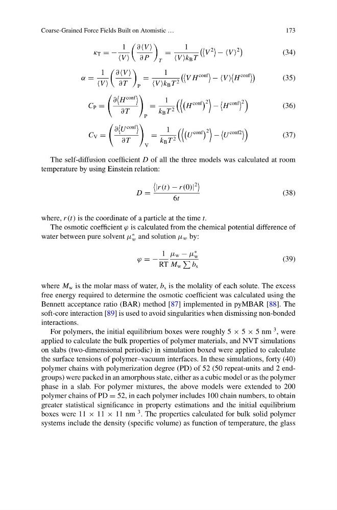
The self-diffusion coefficient D of all the three models was calculated at room
temperature by using Einstein relation:
D =
|r (t) − r (0)|
2
6t
(38)
where, r (t) is the coordinate of a particle at the time t.
The osmotic coefficient ϕ is calculated from the chemical potential difference of
water between pure solvent μ
∗
w and solution μ w by:
ϕ = −
1
RT
μ w − μ
∗
w
M w
b s
(39)
where M w is the molar mass of water, b s is the molality of each solute. The excess
free energy required to determine the osmotic coefficient was calculated using the
Bennett acceptance ratio (BAR) method [87] implemented in pyMBAR [88]. The
soft-core interaction [89] is used to avoid singularities when dismissing non-bonded
interactions.
For polymers, the initial equilibrium boxes were roughly 5 × 5 × 5 nm
3 , were
applied to calculate the bulk properties of polymer materials, and NVT simulations
on slabs (two-dimensional periodic) in simulation boxed were applied to calculate
the surface tensions of polymer–vacuum interfaces. In these simulations, forty (40)
polymer chains with polymerization degree (PD) of 52 (50 repeat-units and 2 endgroups) were packed in an amorphous state, either as a cubic model or as the polymer
phase in a slab. For polymer mixtures, the above models were extended to 200
polymer chains of PD = 52, in each polymer includes 100 chain numbers, to obtain
greater statistical significance in property estimations and the initial equilibrium
boxes were 11 × 11 × 11 nm
3 . The properties calculated for bulk solid polymer
systems include the density (specific volume) as function of temperature, the glass
173
κ T = −
1
V
∂V
∂ P
T
=
1
V k B T
V
2
− V
2
(34)
α =
1
V
∂V
∂ T
P
=
1
V k B T 2
V H
conf
− V
H
conf
(35)
C P =
∂
H
conf
∂ T
P
=
1
k B T 2
H
conf
2
−
H
conf
2
(36)
C V =
∂
U
conf
∂ T
V
=
1
k B T 2
U
conf
2
−
U
conf2
(37)
The self-diffusion coefficient D of all the three models was calculated at room
temperature by using Einstein relation:
D =
|r (t) − r (0)|
2
6t
(38)
where, r (t) is the coordinate of a particle at the time t.
The osmotic coefficient ϕ is calculated from the chemical potential difference of
water between pure solvent μ
∗
w and solution μ w by:
ϕ = −
1
RT
μ w − μ
∗
w
M w
b s
(39)
where M w is the molar mass of water, b s is the molality of each solute. The excess
free energy required to determine the osmotic coefficient was calculated using the
Bennett acceptance ratio (BAR) method [87] implemented in pyMBAR [88]. The
soft-core interaction [89] is used to avoid singularities when dismissing non-bonded
interactions.
For polymers, the initial equilibrium boxes were roughly 5 × 5 × 5 nm
3 , were
applied to calculate the bulk properties of polymer materials, and NVT simulations
on slabs (two-dimensional periodic) in simulation boxed were applied to calculate
the surface tensions of polymer–vacuum interfaces. In these simulations, forty (40)
polymer chains with polymerization degree (PD) of 52 (50 repeat-units and 2 endgroups) were packed in an amorphous state, either as a cubic model or as the polymer
phase in a slab. For polymer mixtures, the above models were extended to 200
polymer chains of PD = 52, in each polymer includes 100 chain numbers, to obtain
greater statistical significance in property estimations and the initial equilibrium
boxes were 11 × 11 × 11 nm
3 . The properties calculated for bulk solid polymer
systems include the density (specific volume) as function of temperature, the glass