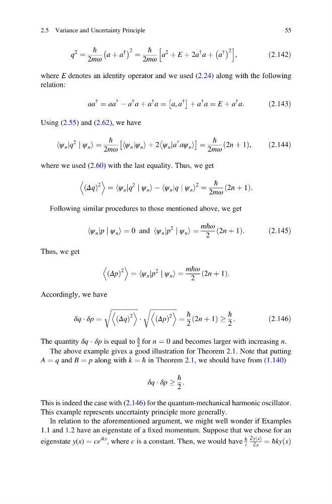
q
2
¼
ħ
2mω
a þ a
{
À
Á 2 ¼
ħ
2mω
a
2
þ E þ 2a
{ a þ a
{
À Á 2
h
i
,
ð2:142Þ
where E denotes an identity operator and we used (2.24) along with the following
relation:
aa
{
¼ aa
{
À a
{ a þ a
{ a ¼ a, a
{
Â
à þ a
{ a ¼ E þ a
{ a:
ð2:143Þ
Using (2.55) and (2.62), we have
ψ n j
h q
2
j ψ n i ¼
ħ
2mω
ψ n j
h ψ n i þ 2 ψ n ja
{ a
ψ n i
Â
à ¼
ħ
2mω
2n þ 1
ð
Þ,
ð2:144Þ
where we used (2.60) with the last equality. Thus, we get
Δq
ð Þ
2
E
D
¼ ψ n j
h q
2
j ψ n i À ψ n j
h q j ψ n i
2 ¼
ħ
2mω
2n þ 1
ð
Þ:
Following similar procedures to those mentioned above, we get
ψ n j
h p j ψ n i ¼ 0 and ψ n j
h p
2
j ψ n i ¼
mħω
2
2n þ 1
ð
Þ:
ð2:145Þ
Thus, we get
Δp
ð Þ
2
E
D
¼ ψ n j
h p
2
j ψ n i ¼
mħω
2
2n þ 1
ð
Þ:
Accordingly, we have
δq Á δp ¼
ffiffiffiffiffiffiffiffiffiffiffiffiffiffiffiffiffi
Δq
ð Þ
2
E
D
r
Á
ffiffiffiffiffiffiffiffiffiffiffiffiffiffiffiffiffi
Δp
ð Þ
2
E
D
r
¼
ħ
2
2n þ 1
ð
Þ!
ħ
2
:
ð2:146Þ
The quantity δq Á δp is equal to
ħ
2 for n ¼ 0 and becomes larger with increasing n.
The above example gives a good illustration for Theorem 2.1. Note that putting
A ¼ q and B ¼ p along with k ¼ ħ in Theorem 2.1, we should have from (1.140)
δq Á δp !
ħ
2
:
This is indeed the case with (2.146) for the quantum-mechanical harmonic oscillator.
This example represents uncertainty principle more generally.
In relation to the aforementioned argument, we might well wonder if Examples
1.1 and 1.2 have an eigenstate of a fixed momentum. Suppose that we chose for an
eigenstate y(x) ¼ ce
ikx , where c is a constant. Then, we would have
ħ
i
∂y x
ð Þ
∂x
¼ ħky x
ð Þ
2.5 Variance and Uncertainty Principle
55