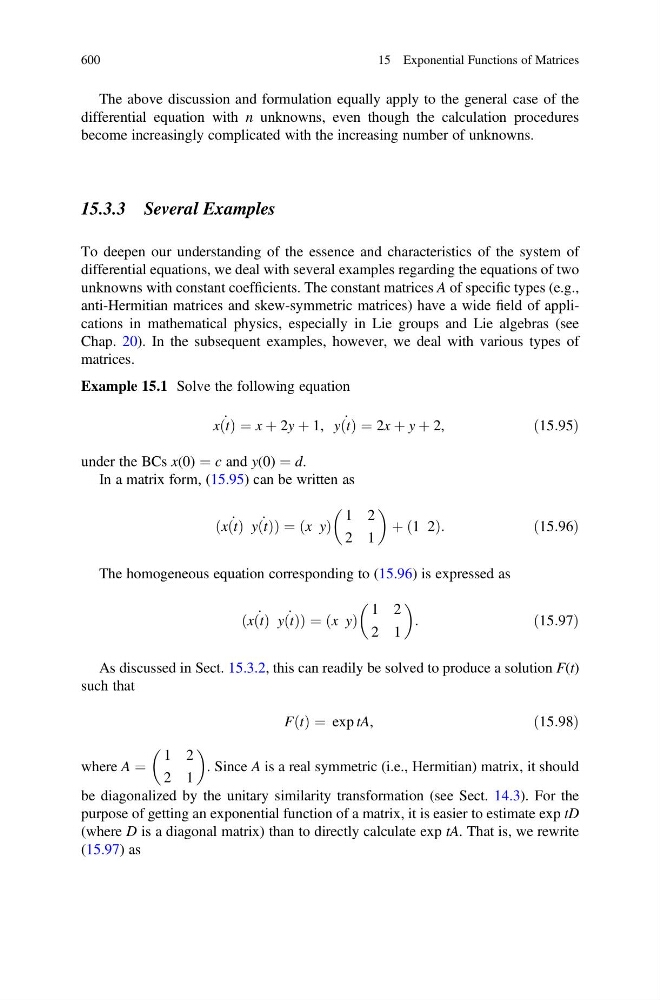
The above discussion and formulation equally apply to the general case of the
differential equation with n unknowns, even though the calculation procedures
become increasingly complicated with the increasing number of unknowns.
15.3.3 Several Examples
To deepen our understanding of the essence and characteristics of the system of
differential equations, we deal with several examples regarding the equations of two
unknowns with constant coefficients. The constant matrices A of specific types (e.g.,
anti-Hermitian matrices and skew-symmetric matrices) have a wide field of applications in mathematical physics, especially in Lie groups and Lie algebras (see
Chap. 20). In the subsequent examples, however, we deal with various types of
matrices.
Example 15.1 Solve the following equation
_
x t
ð Þ ¼ x þ 2y þ 1, _
y t
ð Þ ¼ 2x þ y þ 2,
ð15:95Þ
under the BCs x(0) ¼ c and y(0) ¼ d.
In a matrix form, (15.95) can be written as
ð _
x t
ð Þ _
y t
ð ÞÞ ¼ x y
ð Þ
1 2
2 1
þ 1 2
ð
Þ:
ð15:96Þ
The homogeneous equation corresponding to (15.96) is expressed as
ð _
x t
ð Þ _
y t
ð ÞÞ ¼ x y
ð Þ
1 2
2 1
:
ð15:97Þ
As discussed in Sect. 15.3.2, this can readily be solved to produce a solution F(t)
such that
F t
ð Þ ¼ exp tA,
ð15:98Þ
where A ¼
1 2
2 1
. Since A is a real symmetric (i.e., Hermitian) matrix, it should
be diagonalized by the unitary similarity transformation (see Sect. 14.3). For the
purpose of getting an exponential function of a matrix, it is easier to estimate exp tD
(where D is a diagonal matrix) than to directly calculate exp tA. That is, we rewrite
(15.97) as
600
15 Exponential Functions of Matrices