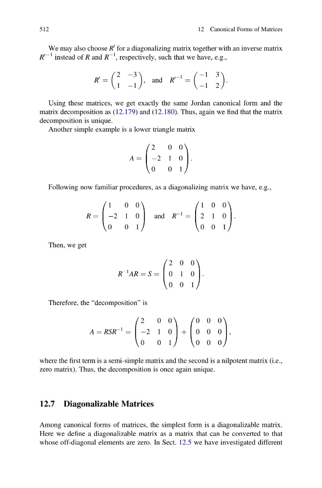
We may also choose R
0 for a diagonalizing matrix together with an inverse matrix
R
0À1 instead of R and R
À1 , respectively, such that we have, e.g.,
R
0
¼
2 À3
1 À1
, and R
0 À1 ¼
À1 3
À1 2
:
Using these matrices, we get exactly the same Jordan canonical form and the
matrix decomposition as (12.179) and (12.180). Thus, again we find that the matrix
decomposition is unique.
Another simple example is a lower triangle matrix
A ¼
2
0 0
À2 1 0
0
0 1
0
B
@
1
C
A:
Following now familiar procedures, as a diagonalizing matrix we have, e.g.,
R ¼
1
0 0
À2 1 0
0
0 1
0
B
@
1
C
A and R
À1
¼
1 0 0
2 1 0
0 0 1
0
B
@
1
C
A:
Then, we get
R
À1 AR ¼ S ¼
2 0 0
0 1 0
0 0 1
0
B
@
1
C
A:
Therefore, the “decomposition” is
A ¼ RSR
À1
¼
2
0 0
À2 1 0
0
0 1
0
B
@
1
C
A þ
0 0 0
0 0 0
0 0 0
0
B
@
1
C
A,
where the first term is a semi-simple matrix and the second is a nilpotent matrix (i.e.,
zero matrix). Thus, the decomposition is once again unique.
12.7 Diagonalizable Matrices
Among canonical forms of matrices, the simplest form is a diagonalizable matrix.
Here we define a diagonalizable matrix as a matrix that can be converted to that
whose off-diagonal elements are zero. In Sect. 12.5 we have investigated different
512
12 Canonical Forms of Matrices