

S ¼
4 0 0 0
0 2 0 0
0 0 2 0
0 0 0 2
0
B
B
B
@
1
C
C
C
A
and N ¼
0 0 0 0
0 0 0 0
0 0 0 1
0 0 0 0
0
B
B
B
@
1
C
C
C
A
,
we have
R
À1 AR ¼ S þ N, i:e:, A ¼ R S þ N
ð
ÞR
À1
¼ RSR
À1
þ RNR
À1
:
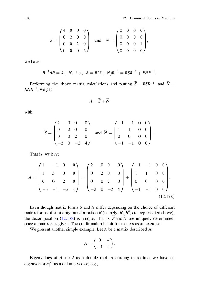
Performing the above matrix calculations and putting e S ¼ RSR
À1 and e
N ¼
RNR
À1 , we get
A ¼ e S þ e
N
with
e S ¼
2
0 0
0
0
2 0
0
0
0 2
0
À2 0 À2 4
0
B
B
B
@
1
C
C
C
A
and e
N ¼
À1 À1 0 0
1
1
0 0
0
0
0 0
À1 À1 0 0
0
B
B
B
@
1
C
C
C
A
:
That is, we have
A ¼
1
À1 0
0
1
3
0
0
0
0
2
0
À3 À1 À2 4
0
B
B
B
B
B
@
1
C
C
C
C
C
A
¼
2
0 0
0
0
2 0
0
0
0 2
0
À2 0 À2 4
0
B
B
B
B
B
@
1
C
C
C
C
C
A
þ
À1 À1 0 0
1
1
0 0
0
0
0 0
À1 À1 0 0
0
B
B
B
B
B
@
1
C
C
C
C
C
A
:
ð12:178Þ
Even though matrix forms S and N differ depending on the choice of different
matrix forms of similarity transformation R (namely, R
0 , R
00
, etc. represented above),
the decomposition (12.178) is unique. That is, e S and e
N are uniquely determined,
once a matrix A is given. The confirmation is left for readers as an exercise.
We present another simple example. Let A be a matrix described as
A ¼
0 4
À1 4
:
Eigenvalues of A are 2 as a double root. According to routine, we have an
eigenvector e
2
ð Þ
1 as a column vector, e.g.,
510
12 Canonical Forms of Matrices
4 0 0 0
0 2 0 0
0 0 2 0
0 0 0 2
0
B
B
B
@
1
C
C
C
A
and N ¼
0 0 0 0
0 0 0 0
0 0 0 1
0 0 0 0
0
B
B
B
@
1
C
C
C
A
,
we have
R
À1 AR ¼ S þ N, i:e:, A ¼ R S þ N
ð
ÞR
À1
¼ RSR
À1
þ RNR
À1
:
Performing the above matrix calculations and putting e S ¼ RSR
À1 and e
N ¼
RNR
À1 , we get
A ¼ e S þ e
N
with
e S ¼
2
0 0
0
0
2 0
0
0
0 2
0
À2 0 À2 4
0
B
B
B
@
1
C
C
C
A
and e
N ¼
À1 À1 0 0
1
1
0 0
0
0
0 0
À1 À1 0 0
0
B
B
B
@
1
C
C
C
A
:
That is, we have
A ¼
1
À1 0
0
1
3
0
0
0
0
2
0
À3 À1 À2 4
0
B
B
B
B
B
@
1
C
C
C
C
C
A
¼
2
0 0
0
0
2 0
0
0
0 2
0
À2 0 À2 4
0
B
B
B
B
B
@
1
C
C
C
C
C
A
þ
À1 À1 0 0
1
1
0 0
0
0
0 0
À1 À1 0 0
0
B
B
B
B
B
@
1
C
C
C
C
C
A
:
ð12:178Þ
Even though matrix forms S and N differ depending on the choice of different
matrix forms of similarity transformation R (namely, R
0 , R
00
, etc. represented above),
the decomposition (12.178) is unique. That is, e S and e
N are uniquely determined,
once a matrix A is given. The confirmation is left for readers as an exercise.
We present another simple example. Let A be a matrix described as
A ¼
0 4
À1 4
:
Eigenvalues of A are 2 as a double root. According to routine, we have an
eigenvector e
2
ð Þ
1 as a column vector, e.g.,
510
12 Canonical Forms of Matrices