

H
h i ¼ ψjHψ
h
i¼ ψ
p
2
2m
ψ
(
)
þ ψ
1
2
mω
2 q
2
ψ
D
E
¼
1
2m
p
{
ψ pψ
j
þ
1
2
mω
2 q
{
ψ qψ
j
¼
1
2m
pψ pψ
j
h
iþ
1
2
mω
2 qψ qψ
j
h
i
¼
1
2m
pψ
k k
2 þ
1
2
mω
2 qψ
k k
2 ! 0,
ð2:13Þ
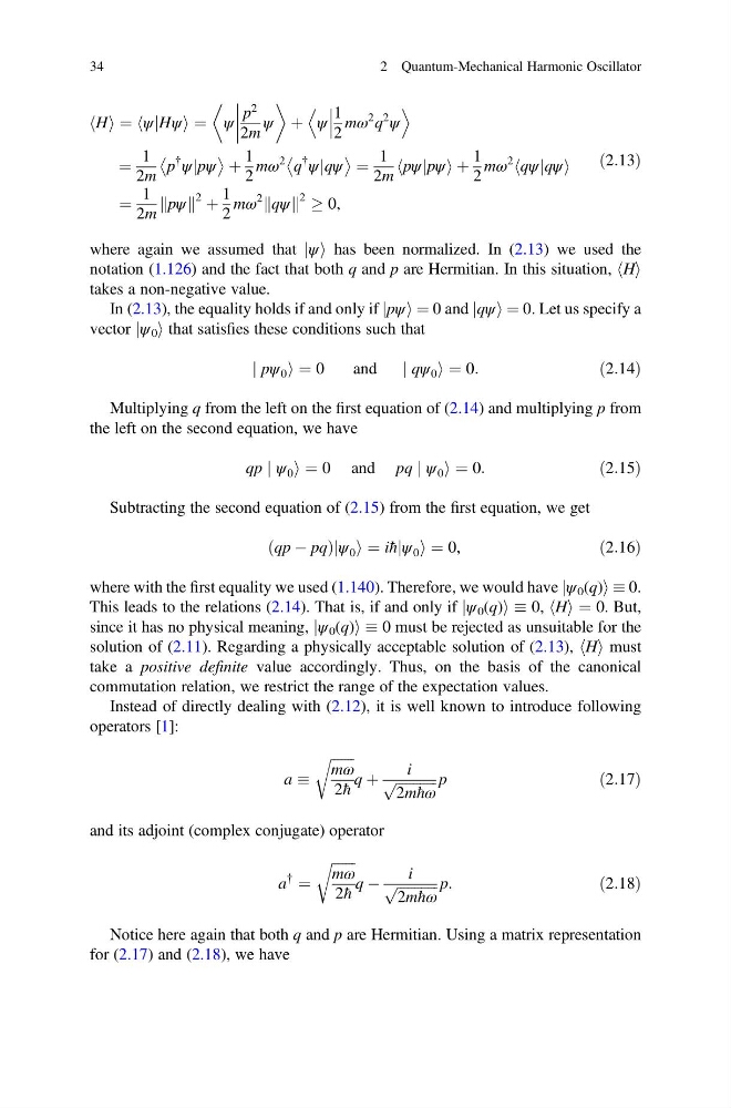
where again we assumed that jψi has been normalized. In (2.13) we used the
notation (1.126) and the fact that both q and p are Hermitian. In this situation, hHi
takes a non-negative value.
In (2.13), the equality holds if and only if jpψi ¼ 0 and jqψi ¼ 0. Let us specify a
vector jψ 0 i that satisfies these conditions such that
j pψ 0 i ¼ 0
and
j qψ 0 i ¼ 0:
ð2:14Þ
Multiplying q from the left on the first equation of (2.14) and multiplying p from
the left on the second equation, we have
qp j ψ 0 i ¼ 0 and pq j ψ 0 i ¼ 0:
ð2:15Þ
Subtracting the second equation of (2.15) from the first equation, we get
qp À pq
ð
Þψ 0 i ¼ iħ
j
j ψ 0 i ¼ 0,
ð2:16Þ
where with the first equality we used (1.140). Therefore, we would have jψ 0 (q)i 0.
This leads to the relations (2.14). That is, if and only if jψ 0 (q)i 0, hHi ¼ 0. But,
since it has no physical meaning, jψ 0 (q)i 0 must be rejected as unsuitable for the
solution of (2.11). Regarding a physically acceptable solution of (2.13), hHi must
take a positive definite value accordingly. Thus, on the basis of the canonical
commutation relation, we restrict the range of the expectation values.
Instead of directly dealing with (2.12), it is well known to introduce following
operators [1]:
a
ffiffiffiffiffiffiffi
mω
2ħ
r
q þ
i
ffiffiffiffiffiffiffiffiffiffiffiffi
2mħω
p
p
ð2:17Þ
and its adjoint (complex conjugate) operator
a
{
¼
ffiffiffiffiffiffiffi
mω
2ħ
r
q À
i
ffiffiffiffiffiffiffiffiffiffiffiffi
2mħω
p
p:
ð2:18Þ
Notice here again that both q and p are Hermitian. Using a matrix representation
for (2.17) and (2.18), we have
34
2 Quantum-Mechanical Harmonic Oscillator
h i ¼ ψjHψ
h
i¼ ψ
p
2
2m
ψ
(
)
þ ψ
1
2
mω
2 q
2
ψ
D
E
¼
1
2m
p
{
ψ pψ
j
þ
1
2
mω
2 q
{
ψ qψ
j
¼
1
2m
pψ pψ
j
h
iþ
1
2
mω
2 qψ qψ
j
h
i
¼
1
2m
pψ
k k
2 þ
1
2
mω
2 qψ
k k
2 ! 0,
ð2:13Þ
where again we assumed that jψi has been normalized. In (2.13) we used the
notation (1.126) and the fact that both q and p are Hermitian. In this situation, hHi
takes a non-negative value.
In (2.13), the equality holds if and only if jpψi ¼ 0 and jqψi ¼ 0. Let us specify a
vector jψ 0 i that satisfies these conditions such that
j pψ 0 i ¼ 0
and
j qψ 0 i ¼ 0:
ð2:14Þ
Multiplying q from the left on the first equation of (2.14) and multiplying p from
the left on the second equation, we have
qp j ψ 0 i ¼ 0 and pq j ψ 0 i ¼ 0:
ð2:15Þ
Subtracting the second equation of (2.15) from the first equation, we get
qp À pq
ð
Þψ 0 i ¼ iħ
j
j ψ 0 i ¼ 0,
ð2:16Þ
where with the first equality we used (1.140). Therefore, we would have jψ 0 (q)i 0.
This leads to the relations (2.14). That is, if and only if jψ 0 (q)i 0, hHi ¼ 0. But,
since it has no physical meaning, jψ 0 (q)i 0 must be rejected as unsuitable for the
solution of (2.11). Regarding a physically acceptable solution of (2.13), hHi must
take a positive definite value accordingly. Thus, on the basis of the canonical
commutation relation, we restrict the range of the expectation values.
Instead of directly dealing with (2.12), it is well known to introduce following
operators [1]:
a
ffiffiffiffiffiffiffi
mω
2ħ
r
q þ
i
ffiffiffiffiffiffiffiffiffiffiffiffi
2mħω
p
p
ð2:17Þ
and its adjoint (complex conjugate) operator
a
{
¼
ffiffiffiffiffiffiffi
mω
2ħ
r
q À
i
ffiffiffiffiffiffiffiffiffiffiffiffi
2mħω
p
p:
ð2:18Þ
Notice here again that both q and p are Hermitian. Using a matrix representation
for (2.17) and (2.18), we have
34
2 Quantum-Mechanical Harmonic Oscillator