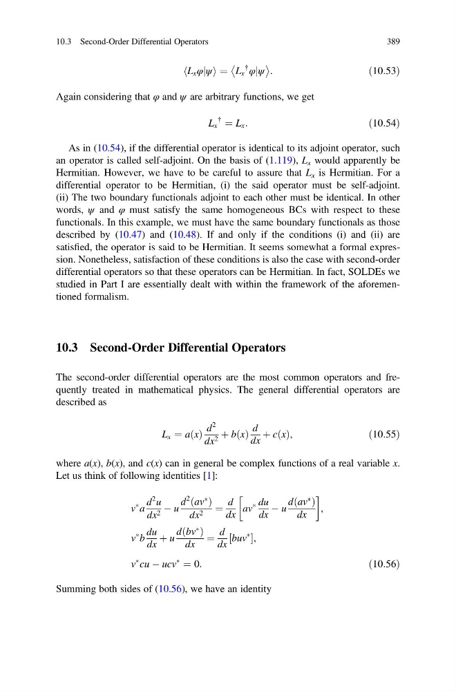
L x φjψ
h
i¼ L x
{
φjψ
:
ð10:53Þ
Again considering that φ and ψ are arbitrary functions, we get
L x
{
¼ L x :
ð10:54Þ
As in (10.54), if the differential operator is identical to its adjoint operator, such
an operator is called self-adjoint. On the basis of (1.119), L x would apparently be
Hermitian. However, we have to be careful to assure that L x is Hermitian. For a
differential operator to be Hermitian, (i) the said operator must be self-adjoint.
(ii) The two boundary functionals adjoint to each other must be identical. In other
words, ψ and φ must satisfy the same homogeneous BCs with respect to these
functionals. In this example, we must have the same boundary functionals as those
described by (10.47) and (10.48). If and only if the conditions (i) and (ii) are
satisfied, the operator is said to be Hermitian. It seems somewhat a formal expression. Nonetheless, satisfaction of these conditions is also the case with second-order
differential operators so that these operators can be Hermitian. In fact, SOLDEs we
studied in Part I are essentially dealt with within the framework of the aforementioned formalism.
10.3 Second-Order Differential Operators
The second-order differential operators are the most common operators and frequently treated in mathematical physics. The general differential operators are
described as
L x ¼ a x
ð Þ
d
2
dx 2 þ b x
ð Þ
d
dx
þ c x
ð Þ,
ð10:55Þ
where a(x), b(x), and c(x) can in general be complex functions of a real variable x.
Let us think of following identities [1]:
v
à a
d
2 u
dx 2 À u
d
2 av
Ã
ð Þ
dx 2 ¼
d
dx
av
à du
dx
À u
d av
Ã
ð Þ
dx
!
,
v
à b
du
dx
þ u
d bv
Ã
ð Þ
dx
¼
d
dx
buv
Ã
½
Š,
v
à cu À ucv
Ã
¼ 0:
ð10:56Þ
Summing both sides of (10.56), we have an identity
10.3 Second-Order Differential Operators
389