

Example 6.12 [6] Evaluate the following real definite integral:
I ¼
Z 1
0
x
aÀ1
1 þ x
dx 0 < a < 1
ð
Þ :
ð6:246Þ
We rewrite (6.246) as
I ¼
Z 1
0
z
aÀ1
1 þ z
dz:
ð6:247Þ
We define the integrand of (6.247) as
f z
ð Þ
z
aÀ1
1 þ z
,
where z
aÀ1 can be further rewritten as
z
aÀ1
¼ e
aÀ1
ð
Þln z
:
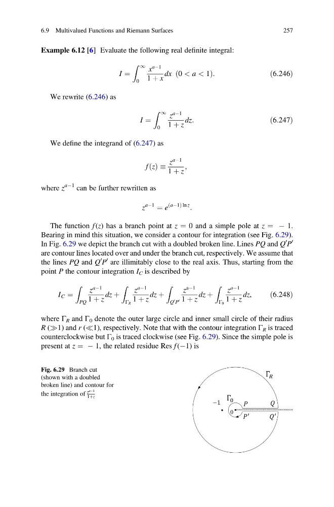
The function f (z) has a branch point at z ¼ 0 and a simple pole at z ¼ À 1.
Bearing in mind this situation, we consider a contour for integration (see Fig. 6.29).
In Fig. 6.29 we depict the branch cut with a doubled broken line. Lines PQ and Q
0 P
0
are contour lines located over and under the branch cut, respectively. We assume that
the lines PQ and Q
0 P
0 are illimitably close to the real axis. Thus, starting from the
point P the contour integration I C is described by
I C ¼
Z
PQ
z
aÀ1
1 þ z
dz þ
Z
Γ R
z
aÀ1
1 þ z
dz þ
Z
Q
0 P
0
z
aÀ1
1 þ z
dz þ
Z
Γ 0
z
aÀ1
1 þ z
dz,
ð6:248Þ
where Γ R and Γ 0 denote the outer large circle and inner small circle of their radius
R ()1) and r ((1), respectively. Note that with the contour integration Γ R is traced
counterclockwise but Γ 0 is traced clockwise (see Fig. 6.29). Since the simple pole is
present at z ¼ À 1, the related residue Res f (À1) is
0
−1
Γ
Γ
Fig. 6.29 Branch cut
(shown with a doubled
broken line) and contour for
the integration of
z
aÀ1
1þz
6.9 Multivalued Functions and Riemann Surfaces
257
I ¼
Z 1
0
x
aÀ1
1 þ x
dx 0 < a < 1
ð
Þ :
ð6:246Þ
We rewrite (6.246) as
I ¼
Z 1
0
z
aÀ1
1 þ z
dz:
ð6:247Þ
We define the integrand of (6.247) as
f z
ð Þ
z
aÀ1
1 þ z
,
where z
aÀ1 can be further rewritten as
z
aÀ1
¼ e
aÀ1
ð
Þln z
:
The function f (z) has a branch point at z ¼ 0 and a simple pole at z ¼ À 1.
Bearing in mind this situation, we consider a contour for integration (see Fig. 6.29).
In Fig. 6.29 we depict the branch cut with a doubled broken line. Lines PQ and Q
0 P
0
are contour lines located over and under the branch cut, respectively. We assume that
the lines PQ and Q
0 P
0 are illimitably close to the real axis. Thus, starting from the
point P the contour integration I C is described by
I C ¼
Z
PQ
z
aÀ1
1 þ z
dz þ
Z
Γ R
z
aÀ1
1 þ z
dz þ
Z
Q
0 P
0
z
aÀ1
1 þ z
dz þ
Z
Γ 0
z
aÀ1
1 þ z
dz,
ð6:248Þ
where Γ R and Γ 0 denote the outer large circle and inner small circle of their radius
R ()1) and r ((1), respectively. Note that with the contour integration Γ R is traced
counterclockwise but Γ 0 is traced clockwise (see Fig. 6.29). Since the simple pole is
present at z ¼ À 1, the related residue Res f (À1) is
0
−1
Γ
Γ
Fig. 6.29 Branch cut
(shown with a doubled
broken line) and contour for
the integration of
z
aÀ1
1þz
6.9 Multivalued Functions and Riemann Surfaces
257