

1 À x
2
À
Á d
2 C
dx
2
À 2 m þ 1
ð
Þx
dC
dx
þ l À m
ð
Þ l þ m þ 1
ð
Þ C ¼ 0 0 m l
ð
Þ : ð3:173Þ
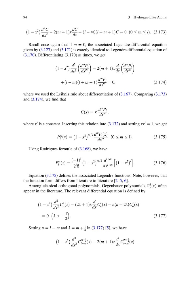
Recall once again that if m ¼ 0, the associated Legendre differential equation
given by (3.127) and (3.171) is exactly identical to Legendre differential equation of
(3.170). Differentiating (3.170) m times, we get
1 À x
2
À
Á d
2
dx
2
d
m P l
dx
m
À 2 m þ 1
ð
Þx
d
dx
d
m P l
dx
m
þ l À m
ð
Þ l þ m þ 1
ð
Þ
d
m P l
dx
m ¼ 0,
ð3:174Þ
where we used the Leibniz rule about differentiation of (3.167). Comparing (3.173)
and (3.174), we find that
C x
ð Þ ¼ κ
0 d
m P l
dx
m ,
where κ
0 is a constant. Inserting this relation into (3.172) and setting κκ
0
¼ 1, we get
P
m
l x
ð Þ ¼ 1 À x
2
À
Á m=2 d
m P l x
ð Þ
dx
m
0 m l
ð
Þ :
ð3:175Þ
Using Rodrigues formula of (3.168), we have
P
m
l x
ð Þ
À1
ð Þ
l
2
l l!
1 À x
2
À
Á m=2 d
lþm
dx lþm 1 À x
2
À
Á l
h
i
:
ð3:176Þ
Equation (3.175) defines the associated Legendre functions. Note, however, that
the function form differs from literature to literature [2, 5, 6].
Among classical orthogonal polynomials, Gegenbauer polynomials C
λ
n x
ð Þ often
appear in the literature. The relevant differential equation is defined by
1 À x
2
À
Á d
2
dx
2
C
λ
n x
ð Þ À 2λ þ 1
ð
Þx
d
dx
C
λ
n x
ð Þ þ n n þ 2λ
ð
ÞC
λ
n x
ð Þ
¼ 0 λ > À
1
2
:
ð3:177Þ
Setting n ¼ l À m and λ ¼ m þ
1
2 in (3.177) [5], we have
1 À x
2
À
Á d
2
dx
2
C
mþ
1
2
lÀm x
ð Þ À 2 m þ 1
ð
Þx
d
dx
C
mþ
1
2
lÀm x
ð Þ
94
3 Hydrogen-Like Atoms
2
À
Á d
2 C
dx
2
À 2 m þ 1
ð
Þx
dC
dx
þ l À m
ð
Þ l þ m þ 1
ð
Þ C ¼ 0 0 m l
ð
Þ : ð3:173Þ
Recall once again that if m ¼ 0, the associated Legendre differential equation
given by (3.127) and (3.171) is exactly identical to Legendre differential equation of
(3.170). Differentiating (3.170) m times, we get
1 À x
2
À
Á d
2
dx
2
d
m P l
dx
m
À 2 m þ 1
ð
Þx
d
dx
d
m P l
dx
m
þ l À m
ð
Þ l þ m þ 1
ð
Þ
d
m P l
dx
m ¼ 0,
ð3:174Þ
where we used the Leibniz rule about differentiation of (3.167). Comparing (3.173)
and (3.174), we find that
C x
ð Þ ¼ κ
0 d
m P l
dx
m ,
where κ
0 is a constant. Inserting this relation into (3.172) and setting κκ
0
¼ 1, we get
P
m
l x
ð Þ ¼ 1 À x
2
À
Á m=2 d
m P l x
ð Þ
dx
m
0 m l
ð
Þ :
ð3:175Þ
Using Rodrigues formula of (3.168), we have
P
m
l x
ð Þ
À1
ð Þ
l
2
l l!
1 À x
2
À
Á m=2 d
lþm
dx lþm 1 À x
2
À
Á l
h
i
:
ð3:176Þ
Equation (3.175) defines the associated Legendre functions. Note, however, that
the function form differs from literature to literature [2, 5, 6].
Among classical orthogonal polynomials, Gegenbauer polynomials C
λ
n x
ð Þ often
appear in the literature. The relevant differential equation is defined by
1 À x
2
À
Á d
2
dx
2
C
λ
n x
ð Þ À 2λ þ 1
ð
Þx
d
dx
C
λ
n x
ð Þ þ n n þ 2λ
ð
ÞC
λ
n x
ð Þ
¼ 0 λ > À
1
2
:
ð3:177Þ
Setting n ¼ l À m and λ ¼ m þ
1
2 in (3.177) [5], we have
1 À x
2
À
Á d
2
dx
2
C
mþ
1
2
lÀm x
ð Þ À 2 m þ 1
ð
Þx
d
dx
C
mþ
1
2
lÀm x
ð Þ
94
3 Hydrogen-Like Atoms