

Y
0
l 0, ϕ
ð
Þ ¼
e
iχ
À1
ð Þ
l
ffiffiffiffiffiffiffiffiffiffiffiffiffiffiffiffi
2l þ 1
ð
Þ
4π
r
P l 1
ð Þ ¼
e
iχ
À1
ð Þ
l
ffiffiffiffiffiffiffiffiffiffiffiffiffiffiffiffi
2l þ 1
ð
Þ
4π
r
,
ð3:147Þ
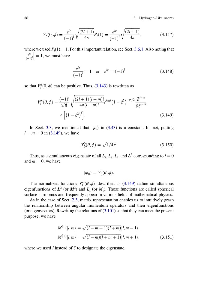
where we used P l (1) ¼ 1. For this important relation, see Sect. 3.6.1. Also noting that
e
iχ
À1
ð Þ
l
¼ 1, we must have
e
iχ
À1
ð Þ
l
¼ 1 or e
iχ
¼ À1
ð Þ
l
ð3:148Þ
so that Y
0
l 0, ϕ
ð
Þ can be positive. Thus, (3.143) is rewritten as
Y
m
l θ, ϕ
ð
Þ ¼
À1
ð Þ
l
2
l l!
ffiffiffiffiffiffiffiffiffiffiffiffiffiffiffiffiffiffiffiffiffiffiffiffiffiffiffiffiffiffiffi ffi
2l þ 1
ð
Þ l þ m
ð
Þ!
4π l À m
ð
Þ!
s
e
imϕ 1 À ξ
2
À
Á Àm=2 ∂
lÀm
∂ξ
lÀm
 1 À ξ
2
À
Á l
h
i
:
ð3:149Þ
In Sect. 3.3, we mentioned that jψ 0 i in (3.43) is a constant. In fact, putting
l ¼ m ¼ 0 in (3.149), we have
Y
0
0 θ, ϕ
ð
Þ ¼
ffiffiffiffiffiffiffiffiffiffi
1=4π
p
:
ð3:150Þ
Thus, as a simultaneous eigenstate of all L x , L y , L z , and L
2 corresponding to l ¼ 0
and m ¼ 0, we have
jψ 0 i Y
0
0 θ, ϕ
ð
Þ:
The normalized functions Y
m
l θ, ϕ
ð
Þ described as (3.149) define simultaneous
eigenfunctions of L
2 (or M
2 ) and L z (or M z ). Those functions are called spherical
surface harmonics and frequently appear in various fields of mathematical physics.
As in the case of Sect. 2.3, matrix representation enables us to intuitively grasp
the relationship between angular momentum operators and their eigenfunctions
(or eigenvectors). Rewriting the relations of (3.101) so that they can meet the present
purpose, we have
M
À
ð Þ
jl, mi ¼
ffiffiffiffiffiffiffiffiffiffiffiffiffiffiffiffiffiffiffiffiffiffiffiffiffiffiffiffiffiffiffiffiffiffiffiffiffi
l À m þ 1
ð
Þl þ m
ð
Þ
p
jl, m À 1i,
M
þ
ð Þ
jl, mi ¼
ffiffiffiffiffiffiffiffiffiffiffiffiffiffiffiffiffiffiffiffiffiffiffiffiffiffiffiffiffiffiffiffiffiffiffiffiffi
l À m
ð
Þ l þ m þ 1
ð
Þ
p
jl, m þ 1i,
ð3:151Þ
where we used l instead of ζ to designate the eigenstate.
86
3 Hydrogen-Like Atoms
0
l 0, ϕ
ð
Þ ¼
e
iχ
À1
ð Þ
l
ffiffiffiffiffiffiffiffiffiffiffiffiffiffiffiffi
2l þ 1
ð
Þ
4π
r
P l 1
ð Þ ¼
e
iχ
À1
ð Þ
l
ffiffiffiffiffiffiffiffiffiffiffiffiffiffiffiffi
2l þ 1
ð
Þ
4π
r
,
ð3:147Þ
where we used P l (1) ¼ 1. For this important relation, see Sect. 3.6.1. Also noting that
e
iχ
À1
ð Þ
l
¼ 1, we must have
e
iχ
À1
ð Þ
l
¼ 1 or e
iχ
¼ À1
ð Þ
l
ð3:148Þ
so that Y
0
l 0, ϕ
ð
Þ can be positive. Thus, (3.143) is rewritten as
Y
m
l θ, ϕ
ð
Þ ¼
À1
ð Þ
l
2
l l!
ffiffiffiffiffiffiffiffiffiffiffiffiffiffiffiffiffiffiffiffiffiffiffiffiffiffiffiffiffiffiffi ffi
2l þ 1
ð
Þ l þ m
ð
Þ!
4π l À m
ð
Þ!
s
e
imϕ 1 À ξ
2
À
Á Àm=2 ∂
lÀm
∂ξ
lÀm
 1 À ξ
2
À
Á l
h
i
:
ð3:149Þ
In Sect. 3.3, we mentioned that jψ 0 i in (3.43) is a constant. In fact, putting
l ¼ m ¼ 0 in (3.149), we have
Y
0
0 θ, ϕ
ð
Þ ¼
ffiffiffiffiffiffiffiffiffiffi
1=4π
p
:
ð3:150Þ
Thus, as a simultaneous eigenstate of all L x , L y , L z , and L
2 corresponding to l ¼ 0
and m ¼ 0, we have
jψ 0 i Y
0
0 θ, ϕ
ð
Þ:
The normalized functions Y
m
l θ, ϕ
ð
Þ described as (3.149) define simultaneous
eigenfunctions of L
2 (or M
2 ) and L z (or M z ). Those functions are called spherical
surface harmonics and frequently appear in various fields of mathematical physics.
As in the case of Sect. 2.3, matrix representation enables us to intuitively grasp
the relationship between angular momentum operators and their eigenfunctions
(or eigenvectors). Rewriting the relations of (3.101) so that they can meet the present
purpose, we have
M
À
ð Þ
jl, mi ¼
ffiffiffiffiffiffiffiffiffiffiffiffiffiffiffiffiffiffiffiffiffiffiffiffiffiffiffiffiffiffiffiffiffiffiffiffiffi
l À m þ 1
ð
Þl þ m
ð
Þ
p
jl, m À 1i,
M
þ
ð Þ
jl, mi ¼
ffiffiffiffiffiffiffiffiffiffiffiffiffiffiffiffiffiffiffiffiffiffiffiffiffiffiffiffiffiffiffiffiffiffiffiffiffi
l À m
ð
Þ l þ m þ 1
ð
Þ
p
jl, m þ 1i,
ð3:151Þ
where we used l instead of ζ to designate the eigenstate.
86
3 Hydrogen-Like Atoms