

6.6 Experimental Equilibrium Structure
145
cancel out. This treatment gives α 1 = 339.791(24) MHz. With the corrected rotational constants, the experimental equilibrium structure has r e (CH) = 109.204 pm
and r e (CO) = 110.558 pm in perfect agreement with the ab initio calculations and a
recent semiexperimental structure: r e (CH) = 109.19(9) pm and r e (CO) = 110.55(3)
pm (Dore et al. 2003).
This example clearly shows the difficulties in obtaining a reliable purely experimental equilibrium structure, even for a small molecule. This case explains why
such structures are only available for very small molecules: Diatomics, triatomics,
tetratomics (NX 3 , PX 3 , AsX 3 , SbH 3 , BiH 3 with X = H, F), and pentatomics (CH 3 X,
SiH 3 X, GeH 3 X with X = F, Cl, Br, I), see Chap. 10.
6.7 Semiexperimental Equilibrium (se) Structure
The semiexperimental method has been employed in many studies and by many
authors (see Vázquez and Stanton (2011) and Mendolicchio et al. (2017) for details),
but it is worth pointing out here that the fundamentals of this technique, yielding an
r
se
e equilibrium structure, were laid down in 1978 by Pulay et al. (1978). Although
they used a very modest Hartree–Fock (HF) level of theory, they could determine
an accurate SE structure of methane, CH 4 , with r e = 108.62(5) pm, which was
later improved and confirmed by the almost perfect agreement of the SE structure
and the one computed at a high level of ab initio theory [r e = 108.595(30) pm]
(Stanton 1999). The pioneering work of Allen et al. (1990, 1992), Clabo et al. (1988)
must be quoted because they were among the first workers to determine accurate
semiexperimental structures, for instance for HNCO (East et al. 1993) and ketene,
CH 2 =C=O, (East and Allen 1995).
As the determination of an experimental equilibrium structure is extremely
complicated and time-consuming, it is attractive to calculate the rovibrational correction from the anharmonic force field. This method avoids the problem of measuring
rotational constants of excited vibrational states of all needed isotopologues. Furthermore, the difficulty originating from the anharmonic resonances disappears. Finally,
the summation of the α-constants eliminates the (possibly small) denominator in the
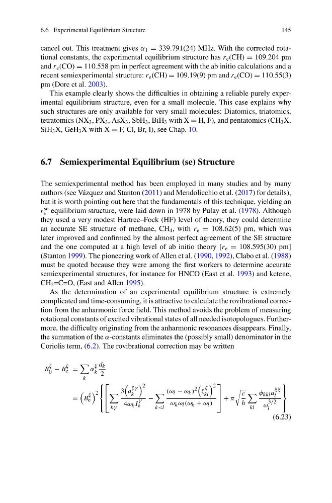
Coriolis term, (6.2). The rovibrational correction may be written
B
ξ
0 − B
ξ
e =
k
α
ξ
k
d k
2
=
B
ξ
e
2
⎧
⎪ ⎨
⎪ ⎩
⎡
⎢
⎣
kγ
3
a
ξγ
k
2
4ω k I
γ
e
−
k
ζ
ξ
kl
2
ω k ω l (ω k + ω l )
⎤
⎥
⎦ + π
c
h
kl
φ kkl a
ξξ
l
ω
3/2
l
⎫
⎪ ⎬
⎪ ⎭
(6.23)
145
cancel out. This treatment gives α 1 = 339.791(24) MHz. With the corrected rotational constants, the experimental equilibrium structure has r e (CH) = 109.204 pm
and r e (CO) = 110.558 pm in perfect agreement with the ab initio calculations and a
recent semiexperimental structure: r e (CH) = 109.19(9) pm and r e (CO) = 110.55(3)
pm (Dore et al. 2003).
This example clearly shows the difficulties in obtaining a reliable purely experimental equilibrium structure, even for a small molecule. This case explains why
such structures are only available for very small molecules: Diatomics, triatomics,
tetratomics (NX 3 , PX 3 , AsX 3 , SbH 3 , BiH 3 with X = H, F), and pentatomics (CH 3 X,
SiH 3 X, GeH 3 X with X = F, Cl, Br, I), see Chap. 10.
6.7 Semiexperimental Equilibrium (se) Structure
The semiexperimental method has been employed in many studies and by many
authors (see Vázquez and Stanton (2011) and Mendolicchio et al. (2017) for details),
but it is worth pointing out here that the fundamentals of this technique, yielding an
r
se
e equilibrium structure, were laid down in 1978 by Pulay et al. (1978). Although
they used a very modest Hartree–Fock (HF) level of theory, they could determine
an accurate SE structure of methane, CH 4 , with r e = 108.62(5) pm, which was
later improved and confirmed by the almost perfect agreement of the SE structure
and the one computed at a high level of ab initio theory [r e = 108.595(30) pm]
(Stanton 1999). The pioneering work of Allen et al. (1990, 1992), Clabo et al. (1988)
must be quoted because they were among the first workers to determine accurate
semiexperimental structures, for instance for HNCO (East et al. 1993) and ketene,
CH 2 =C=O, (East and Allen 1995).
As the determination of an experimental equilibrium structure is extremely
complicated and time-consuming, it is attractive to calculate the rovibrational correction from the anharmonic force field. This method avoids the problem of measuring
rotational constants of excited vibrational states of all needed isotopologues. Furthermore, the difficulty originating from the anharmonic resonances disappears. Finally,
the summation of the α-constants eliminates the (possibly small) denominator in the
Coriolis term, (6.2). The rovibrational correction may be written
B
ξ
0 − B
ξ
e =
k
α
ξ
k
d k
2
=
B
ξ
e
2
⎧
⎪ ⎨
⎪ ⎩
⎡
⎢
⎣
kγ
3
a
ξγ
k
2
4ω k I
γ
e
−
k
ζ
ξ
kl
2
ω k ω l (ω k + ω l )
⎤
⎥
⎦ + π
c
h
kl
φ kkl a
ξξ
l
ω
3/2
l
⎫
⎪ ⎬
⎪ ⎭
(6.23)