

(1) Sum of squares between microcosms S AB ¼
P
ij c
À
y ij: À
y ...
Á 2
(2) Sum of squares between populations S A ¼
P
i bc
À
y i:: À
y ...
Á 2
(3) Sum of squares in a population
S B(A) ¼ S AB À S A
(4) Sum of squares of time and population S AC ¼
P
ik b
À
y i:k À
y ...
Á 2
(5) Sum of squares between times S C ¼
P
k ab
À
y ::k À
y ...
Á 2
(6) Sum of squares of time  population S A  C ¼ S AC À S A À S C
(7) Total sum of squares
S T ¼
P
ijk
À
y ijk À
y ...
Á 2
(8) Sum of squared error
S E ¼ S T À S AB À S C À S A Â C
– Procedure (3): Calculate the degrees of freedom using the following expressions
(1–7). Here, the flexibility is defined as various statistics. For example, the
flexibility of the observation data with sample size n (x 1 , x 2 ,. . .. . ., x n ) becomes n:
(1) ν A ¼ a À 1
(2) ν B(A) ¼ a(b À 1)
(3) ν AB ¼ ab À 1
(4) ν c ¼ c À 1
(5) ν A Â C ¼ (a À 1)(c À 1)
(6) ν E ¼ abc À 1 À ν AB À ν C À ν A Â C
(7) ν T ¼ ν A + ν B(A) + ν C + ν A Â C + ν E
– Procedure (4): Calculate the unbiased variance using the following expressions
(1–5), where (3) is the value of the sum of squares divided by the degree of
freedom.
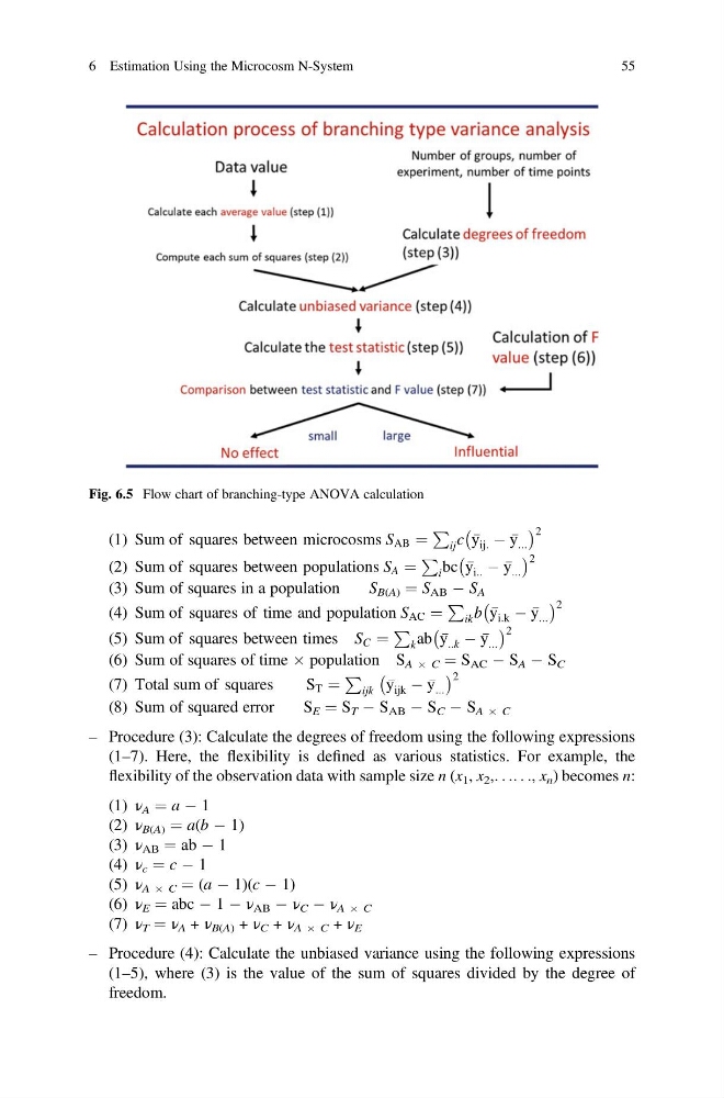
Fig. 6.5 Flow chart of branching-type ANOVA calculation
6 Estimation Using the Microcosm N-System
55
P
ij c
À
y ij: À
y ...
Á 2
(2) Sum of squares between populations S A ¼
P
i bc
À
y i:: À
y ...
Á 2
(3) Sum of squares in a population
S B(A) ¼ S AB À S A
(4) Sum of squares of time and population S AC ¼
P
ik b
À
y i:k À
y ...
Á 2
(5) Sum of squares between times S C ¼
P
k ab
À
y ::k À
y ...
Á 2
(6) Sum of squares of time  population S A  C ¼ S AC À S A À S C
(7) Total sum of squares
S T ¼
P
ijk
À
y ijk À
y ...
Á 2
(8) Sum of squared error
S E ¼ S T À S AB À S C À S A Â C
– Procedure (3): Calculate the degrees of freedom using the following expressions
(1–7). Here, the flexibility is defined as various statistics. For example, the
flexibility of the observation data with sample size n (x 1 , x 2 ,. . .. . ., x n ) becomes n:
(1) ν A ¼ a À 1
(2) ν B(A) ¼ a(b À 1)
(3) ν AB ¼ ab À 1
(4) ν c ¼ c À 1
(5) ν A Â C ¼ (a À 1)(c À 1)
(6) ν E ¼ abc À 1 À ν AB À ν C À ν A Â C
(7) ν T ¼ ν A + ν B(A) + ν C + ν A Â C + ν E
– Procedure (4): Calculate the unbiased variance using the following expressions
(1–5), where (3) is the value of the sum of squares divided by the degree of
freedom.
Fig. 6.5 Flow chart of branching-type ANOVA calculation
6 Estimation Using the Microcosm N-System
55