

How to Reduce Computation Time
75
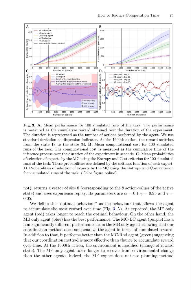
Fig. 3. A. Mean performance for 100 simulated runs of the task. The performance
is measured as the cumulative reward obtained over the duration of the experiment.
The duration is represented as the number of actions performed by the agent. We use
standard deviation as dispersion indicator. At the 1600th action, the reward switches
from the state 18 to the state 34. B. Mean computational cost for 100 simulated
runs of the task. The computational cost is measured as the cumulative time of the
inference process over the duration of the experiment in seconds. C. Mean probabilities
of selection of experts by the MC using the Entropy and Cost criterion for 100 simulated
runs of the task. These probabilities are defined by the softmax function of each expert.
D. Probabilities of selection of experts by the MC using the Entropy and Cost criterion
for 2 simulated runs of the task. (Color figure online)
not), returns a vector of size 8 (corresponding to the 8 action-values of the active
state) and uses experience replay. Its parameters are α = 0.1 γ = 0.95 and τ =
0.05.
We define the “optimal behaviour” as the behaviour that allows the agent
to accumulate the most reward over time (Fig. 3. A). As expected, the MF only
agent (red) takes longer to reach the optimal behaviour. On the other hand, the
MB only agent (blue) has the best performance. The MC-EC agent (purple) has a
non-significantly different performance from the MB only agent, showing that our
coordination method does not penalize the agent in terms of cumulated reward.
In addition to that, it performs better than the MC-Rnd agent (green) suggesting
that our coordination method is more effective than chance to accumulate reward
over time. At the 1600th action, the environment is modified (change of reward
state). The MF only agent takes longer to recover from environmental change
than the other agents. Indeed, the MF expert does not use planning method
75
Fig. 3. A. Mean performance for 100 simulated runs of the task. The performance
is measured as the cumulative reward obtained over the duration of the experiment.
The duration is represented as the number of actions performed by the agent. We use
standard deviation as dispersion indicator. At the 1600th action, the reward switches
from the state 18 to the state 34. B. Mean computational cost for 100 simulated
runs of the task. The computational cost is measured as the cumulative time of the
inference process over the duration of the experiment in seconds. C. Mean probabilities
of selection of experts by the MC using the Entropy and Cost criterion for 100 simulated
runs of the task. These probabilities are defined by the softmax function of each expert.
D. Probabilities of selection of experts by the MC using the Entropy and Cost criterion
for 2 simulated runs of the task. (Color figure online)
not), returns a vector of size 8 (corresponding to the 8 action-values of the active
state) and uses experience replay. Its parameters are α = 0.1 γ = 0.95 and τ =
0.05.
We define the “optimal behaviour” as the behaviour that allows the agent
to accumulate the most reward over time (Fig. 3. A). As expected, the MF only
agent (red) takes longer to reach the optimal behaviour. On the other hand, the
MB only agent (blue) has the best performance. The MC-EC agent (purple) has a
non-significantly different performance from the MB only agent, showing that our
coordination method does not penalize the agent in terms of cumulated reward.
In addition to that, it performs better than the MC-Rnd agent (green) suggesting
that our coordination method is more effective than chance to accumulate reward
over time. At the 1600th action, the environment is modified (change of reward
state). The MF only agent takes longer to recover from environmental change
than the other agents. Indeed, the MF expert does not use planning method