

13 Computational Biomechanics of the Brain in the Operating Theatre
333
of E = 10 kPa is used for the tumour. To take into account large displacements
while being computationally efficient, simulations are run using the corotational
approach [34].
13.3.3.2 Constraints
Two types of constraints are used during the registration process:
• Bilateral constraints (δ = 0) used to impose displacement such that constrained
points of the model are moved to a desired position.
• Unilateral constraints (δ ⊥ λ i.e. δ ≥ 0 and λ ≥ 0 and δ · λ = 0) are used
to impose contacts between structures. In other words, either the violation is
positive (δ ≥ 0) and no contact forces are applied (λ = 0) or the violation
must be nullified (δ = 0) with a positive constraint force (λ ≥ 0).
Due to the nonlinearity of H, a unique solution does not exist. Instead, we use
an iterative method where the problem is linearised at each iteration, allowing for
the convergence towards the closest local minimum. Constraint equations are then
defined at the beginning of each iteration using the current position of the model and
are assumed to be constant during the solving process H(u col , p I ) ∂H/∂u = H.
The constraint matrix H (known as the Jacobian of the constraints) contains the
directions on which Lagrangian multipliers are computed.
For each iteration i, a single iteration of a Newton-Raphson method is solved,
while constraint equations are defined following an iterative closest point (ICP)
algorithm [35]. Each point extracted from the intra-operative data is associated
with its closest element on the biomechanical model (see Sect. 13.3.4), defining this
way the directions (stored in the matrix H i ) in which constraint forces λ are applied
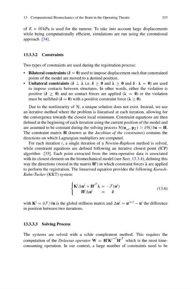
to perform the registration. The linearised equation provides the following KarushKuhn-Tucker (KKT) system:
K i u i + H i T λ = −F(u i )
H i u i
=
δ
(13.6)
with K i = ∂F/∂u is the global stiffness matrix and u i = u i+1 − u i the difference
in position between two iterations.
13.3.3.3 Solving Process
The systems are solved with a schür complement method. This requires the
computation of the Delassus operator W = H i K i −1 H i T which is the most timeconsuming operation. In our context, a large number of constraints need to be
333
of E = 10 kPa is used for the tumour. To take into account large displacements
while being computationally efficient, simulations are run using the corotational
approach [34].
13.3.3.2 Constraints
Two types of constraints are used during the registration process:
• Bilateral constraints (δ = 0) used to impose displacement such that constrained
points of the model are moved to a desired position.
• Unilateral constraints (δ ⊥ λ i.e. δ ≥ 0 and λ ≥ 0 and δ · λ = 0) are used
to impose contacts between structures. In other words, either the violation is
positive (δ ≥ 0) and no contact forces are applied (λ = 0) or the violation
must be nullified (δ = 0) with a positive constraint force (λ ≥ 0).
Due to the nonlinearity of H, a unique solution does not exist. Instead, we use
an iterative method where the problem is linearised at each iteration, allowing for
the convergence towards the closest local minimum. Constraint equations are then
defined at the beginning of each iteration using the current position of the model and
are assumed to be constant during the solving process H(u col , p I ) ∂H/∂u = H.
The constraint matrix H (known as the Jacobian of the constraints) contains the
directions on which Lagrangian multipliers are computed.
For each iteration i, a single iteration of a Newton-Raphson method is solved,
while constraint equations are defined following an iterative closest point (ICP)
algorithm [35]. Each point extracted from the intra-operative data is associated
with its closest element on the biomechanical model (see Sect. 13.3.4), defining this
way the directions (stored in the matrix H i ) in which constraint forces λ are applied
to perform the registration. The linearised equation provides the following KarushKuhn-Tucker (KKT) system:
K i u i + H i T λ = −F(u i )
H i u i
=
δ
(13.6)
with K i = ∂F/∂u is the global stiffness matrix and u i = u i+1 − u i the difference
in position between two iterations.
13.3.3.3 Solving Process
The systems are solved with a schür complement method. This requires the
computation of the Delassus operator W = H i K i −1 H i T which is the most timeconsuming operation. In our context, a large number of constraints need to be