

11 Meshless Algorithms for Computational Biomechanics of the Brain
287
robust, computationally efficient and suitable for application in surgery simulation
where the users are unlikely to have expert knowledge of computational mechanics.
Therefore, we offer no recommendation regarding the method of choice for 3-D
computational biomechanics modelling of surgical dissection and rupture propagation.
11.5 Stability of Explicit Dynamics Meshless Algorithms
For Computation of Soft Tissue Deformation
Both the Meshless Total Lagrangian Explicit Dynamics (MTLED) framework
discussed here and the Total Lagrangian Explicit Dynamics (TLED) finite element
algorithm for neurosurgical simulation described in Chap. 10 use the central
difference method for time stepping. This method is only conditionally stable. The
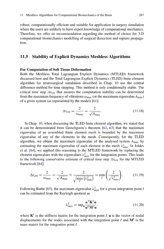
critical time step Δt crit that ensures the computation stability can be determined
from the maximum frequency of vibrations ω max (or the maximum eigenvalue A max )
of a given system (as represented by the model) [61]:
t crit =
2
ω max
=
2
√
A max
.
(11.18)
In Chap. 10, when discussing the TLED finite element algorithm, we stated that
it can be demonstrated from Gerschgorin’s theorem [62, 63] that the maximum
eigenvalue of an assembled finite element mesh is bounded by the maximum
eigenvalue of any of the elements in the mesh. Consequently, for the TLED
algorithm, we obtain the maximum eigenvalue of the analysed system A max by
estimating the maximum eigenvalue of each element in the mesh λ e
max . In Joldes
et al. [64], we applied this reasoning to the MTLED framework by replacing the
element eigenvalues with the eigenvalues λ I
max for the integration points. This leads
to the following conservative estimate of critical time step t crit for the MTLED
framework [64]:
t crit =
2
ω max
=
2
√
A max
≈
2
max
I
λ I
max
= min
I
2
λ I
max
.
(11.19)
Following Bathe [65], the maximum eigenvalue λ I
max for a given integration point I
can be estimated from the Rayleigh quotient as
λ
I
max = sup u
u T K I u
u T M I u
,
(11.20)
where K I is the stiffness matrix for the integration point I, u is the vector of nodal
displacements for the nodes associated with the integration point I and M I is the
mass matrix for the integration point I.
287
robust, computationally efficient and suitable for application in surgery simulation
where the users are unlikely to have expert knowledge of computational mechanics.
Therefore, we offer no recommendation regarding the method of choice for 3-D
computational biomechanics modelling of surgical dissection and rupture propagation.
11.5 Stability of Explicit Dynamics Meshless Algorithms
For Computation of Soft Tissue Deformation
Both the Meshless Total Lagrangian Explicit Dynamics (MTLED) framework
discussed here and the Total Lagrangian Explicit Dynamics (TLED) finite element
algorithm for neurosurgical simulation described in Chap. 10 use the central
difference method for time stepping. This method is only conditionally stable. The
critical time step Δt crit that ensures the computation stability can be determined
from the maximum frequency of vibrations ω max (or the maximum eigenvalue A max )
of a given system (as represented by the model) [61]:
t crit =
2
ω max
=
2
√
A max
.
(11.18)
In Chap. 10, when discussing the TLED finite element algorithm, we stated that
it can be demonstrated from Gerschgorin’s theorem [62, 63] that the maximum
eigenvalue of an assembled finite element mesh is bounded by the maximum
eigenvalue of any of the elements in the mesh. Consequently, for the TLED
algorithm, we obtain the maximum eigenvalue of the analysed system A max by
estimating the maximum eigenvalue of each element in the mesh λ e
max . In Joldes
et al. [64], we applied this reasoning to the MTLED framework by replacing the
element eigenvalues with the eigenvalues λ I
max for the integration points. This leads
to the following conservative estimate of critical time step t crit for the MTLED
framework [64]:
t crit =
2
ω max
=
2
√
A max
≈
2
max
I
λ I
max
= min
I
2
λ I
max
.
(11.19)
Following Bathe [65], the maximum eigenvalue λ I
max for a given integration point I
can be estimated from the Rayleigh quotient as
λ
I
max = sup u
u T K I u
u T M I u
,
(11.20)
where K I is the stiffness matrix for the integration point I, u is the vector of nodal
displacements for the nodes associated with the integration point I and M I is the
mass matrix for the integration point I.