

11 Meshless Algorithms for Computational Biomechanics of the Brain
283
• New integration points are introduced only in the areas where the integration
accuracy is below the desired (required) accuracy.
• The scheme works for any shape and size of support domains.
• The scheme is particularly effective for irregular/non-uniform nodal distributions.
In practice, defining the relative integration tolerance τ is the only input required
from the analyst for the adaptive integration scheme used in the MTLED framework.
Although it is rather difficult to formulate detailed guidelines regarding selection
of such tolerance, the numerical experiments we conducted in Joldes et al. [21]
have indicated that the solution accuracy does not appreciably increase after the
integration accuracy reaches a certain level/threshold. This, in turn, suggests that it
is not necessary to use very high integration accuracy (low tolerance τ ) resulting in
many subdivisions of each integrationcell.
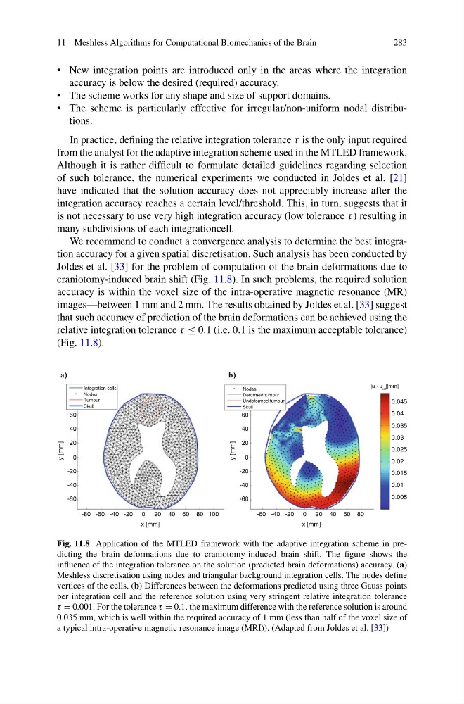
We recommend to conduct a convergence analysis to determine the best integration accuracy for a given spatial discretisation. Such analysis has been conducted by
Joldes et al. [33] for the problem of computation of the brain deformations due to
craniotomy-induced brain shift (Fig. 11.8). In such problems, the required solution
accuracy is within the voxel size of the intra-operative magnetic resonance (MR)
images—between 1 mm and 2 mm. The results obtained by Joldes et al. [33] suggest
that such accuracy of prediction of the brain deformations can be achieved using the
relative integration tolerance τ ≤ 0.1 (i.e. 0.1 is the maximum acceptable tolerance)
(Fig. 11.8).
60
60
40
40
100
80
20
20
x [mm]
y [mm]
Integration cells
Nodes
Tumour
Skull
Nodes
b)
a)
Deformed tumour
Undeformed tumour
Skull
-20
-20
-40
-40
-60
-60
-80
0
0
60
60
40
40
80
0.005
0.01
0.015
0.02
0.025
0.03
0.035
0.04
0.045
|u - u ref |[mm]
20
20
x [mm]
y [mm]
-20
-20
-40
-40
-60
-60
0
0
Fig. 11.8 Application of the MTLED framework with the adaptive integration scheme in predicting the brain deformations due to craniotomy-induced brain shift. The figure shows the
influence of the integration tolerance on the solution (predicted brain deformations) accuracy. (a)
Meshless discretisation using nodes and triangular background integration cells. The nodes define
vertices of the cells. (b) Differences between the deformations predicted using three Gauss points
per integration cell and the reference solution using very stringent relative integration tolerance
τ = 0.001. For the tolerance τ = 0.1, the maximum difference with the reference solution is around
0.035 mm, which is well within the required accuracy of 1 mm (less than half of the voxel size of
a typical intra-operative magnetic resonance image (MRI)). (Adapted from Joldes et al. [33])
283
• New integration points are introduced only in the areas where the integration
accuracy is below the desired (required) accuracy.
• The scheme works for any shape and size of support domains.
• The scheme is particularly effective for irregular/non-uniform nodal distributions.
In practice, defining the relative integration tolerance τ is the only input required
from the analyst for the adaptive integration scheme used in the MTLED framework.
Although it is rather difficult to formulate detailed guidelines regarding selection
of such tolerance, the numerical experiments we conducted in Joldes et al. [21]
have indicated that the solution accuracy does not appreciably increase after the
integration accuracy reaches a certain level/threshold. This, in turn, suggests that it
is not necessary to use very high integration accuracy (low tolerance τ ) resulting in
many subdivisions of each integrationcell.
We recommend to conduct a convergence analysis to determine the best integration accuracy for a given spatial discretisation. Such analysis has been conducted by
Joldes et al. [33] for the problem of computation of the brain deformations due to
craniotomy-induced brain shift (Fig. 11.8). In such problems, the required solution
accuracy is within the voxel size of the intra-operative magnetic resonance (MR)
images—between 1 mm and 2 mm. The results obtained by Joldes et al. [33] suggest
that such accuracy of prediction of the brain deformations can be achieved using the
relative integration tolerance τ ≤ 0.1 (i.e. 0.1 is the maximum acceptable tolerance)
(Fig. 11.8).
60
60
40
40
100
80
20
20
x [mm]
y [mm]
Integration cells
Nodes
Tumour
Skull
Nodes
b)
a)
Deformed tumour
Undeformed tumour
Skull
-20
-20
-40
-40
-60
-60
-80
0
0
60
60
40
40
80
0.005
0.01
0.015
0.02
0.025
0.03
0.035
0.04
0.045
|u - u ref |[mm]
20
20
x [mm]
y [mm]
-20
-20
-40
-40
-60
-60
0
0
Fig. 11.8 Application of the MTLED framework with the adaptive integration scheme in predicting the brain deformations due to craniotomy-induced brain shift. The figure shows the
influence of the integration tolerance on the solution (predicted brain deformations) accuracy. (a)
Meshless discretisation using nodes and triangular background integration cells. The nodes define
vertices of the cells. (b) Differences between the deformations predicted using three Gauss points
per integration cell and the reference solution using very stringent relative integration tolerance
τ = 0.001. For the tolerance τ = 0.1, the maximum difference with the reference solution is around
0.035 mm, which is well within the required accuracy of 1 mm (less than half of the voxel size of
a typical intra-operative magnetic resonance image (MRI)). (Adapted from Joldes et al. [33])