

2.4 Approximate Methods for Solving the Transport Equation
17
• the error does not affect the dimension of the problem;
• simple structure of the computational algorithm;
From the viewpoint of the solutions of the equation for radiative transfer the
Monte-Carlo method is a computer simulation of the random motion of N photons
[14]. To obtain reasonable approximation to one have consider a large number of
photons because the accuracy of the results is proportional to
√
N . The main idea
of the method is the registration of effects of absorption and scattering throughout
the optical path of a photon through a non-transparent environment. The distance
between two collisions is chosen from a logarithmic distribution, using a random
number generated by a computer. To take into account absorption, each photon is
assigned a weight.
If there is scattering, a new direction propagation is chosen according to phase
function and other random number. This procedure is repeated as long as the photon
does not come out of the considered volume or the weight reaches a certain value.
The Monte-Carlo method includes five main steps: generation of the source photon
trajectory, absorption, destruction, registration [14].
1. Generation of photon source. The photons are generated on the surface of the
medium. Their spatial and angular distribution corresponds to the distribution
of the incident radiation (for example, a Gaussian beam).
2. The generation of the trajectory. After generation of a photon the distance to
the first collision is determined. We expect that the absorbing and scattering
particles are randomly distributed in opaque medium. Then, the value of free
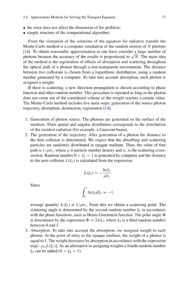
path is 1/ρσ x , where ρ is particle number density and σ x is the scattering crosssection. Random number 0 < ξ 1 < 1 is generated by computer and the distance
to the next collision L(ξ 1 ) is calculated from the expression
L(ξ 1 ) = −
ln ξ 1
ρσ x
.
Since
1
0
ln ξ 1 dξ 1 = −1,
average quantity L(ξ 1 ) is 1/ρσ x . From this we obtain a scattering point. The
scattering angle is determined by the second random number ξ 2 in accordance
with the phase functions, such as Henie-Greenstein function. The polar angle
is determined by the expression = 2πξ 3 , where ξ 3 is a third random number
between 0 and 1.
3. Absorption. To take into account the absorption, we assigned weight to each
photon. At the point of entry to the opaque medium, the weight of a photon is
equal to 1. The weight decreases by absorption in accordance with the expression
exp[−μ a L(ξ 1 )]. As an alternative to assigning weights a fourth random number
ξ 4 can be added (0 < ξ 4 < 1).
17
• the error does not affect the dimension of the problem;
• simple structure of the computational algorithm;
From the viewpoint of the solutions of the equation for radiative transfer the
Monte-Carlo method is a computer simulation of the random motion of N photons
[14]. To obtain reasonable approximation to one have consider a large number of
photons because the accuracy of the results is proportional to
√
N . The main idea
of the method is the registration of effects of absorption and scattering throughout
the optical path of a photon through a non-transparent environment. The distance
between two collisions is chosen from a logarithmic distribution, using a random
number generated by a computer. To take into account absorption, each photon is
assigned a weight.
If there is scattering, a new direction propagation is chosen according to phase
function and other random number. This procedure is repeated as long as the photon
does not come out of the considered volume or the weight reaches a certain value.
The Monte-Carlo method includes five main steps: generation of the source photon
trajectory, absorption, destruction, registration [14].
1. Generation of photon source. The photons are generated on the surface of the
medium. Their spatial and angular distribution corresponds to the distribution
of the incident radiation (for example, a Gaussian beam).
2. The generation of the trajectory. After generation of a photon the distance to
the first collision is determined. We expect that the absorbing and scattering
particles are randomly distributed in opaque medium. Then, the value of free
path is 1/ρσ x , where ρ is particle number density and σ x is the scattering crosssection. Random number 0 < ξ 1 < 1 is generated by computer and the distance
to the next collision L(ξ 1 ) is calculated from the expression
L(ξ 1 ) = −
ln ξ 1
ρσ x
.
Since
1
0
ln ξ 1 dξ 1 = −1,
average quantity L(ξ 1 ) is 1/ρσ x . From this we obtain a scattering point. The
scattering angle is determined by the second random number ξ 2 in accordance
with the phase functions, such as Henie-Greenstein function. The polar angle
is determined by the expression = 2πξ 3 , where ξ 3 is a third random number
between 0 and 1.
3. Absorption. To take into account the absorption, we assigned weight to each
photon. At the point of entry to the opaque medium, the weight of a photon is
equal to 1. The weight decreases by absorption in accordance with the expression
exp[−μ a L(ξ 1 )]. As an alternative to assigning weights a fourth random number
ξ 4 can be added (0 < ξ 4 < 1).