

6.4 Matrix Formulation of Scattering for the jth Bilayer …
113
6.4 Matrix Formulation of Scattering for the j th Bilayer
Particle of an Arbitrary Shape
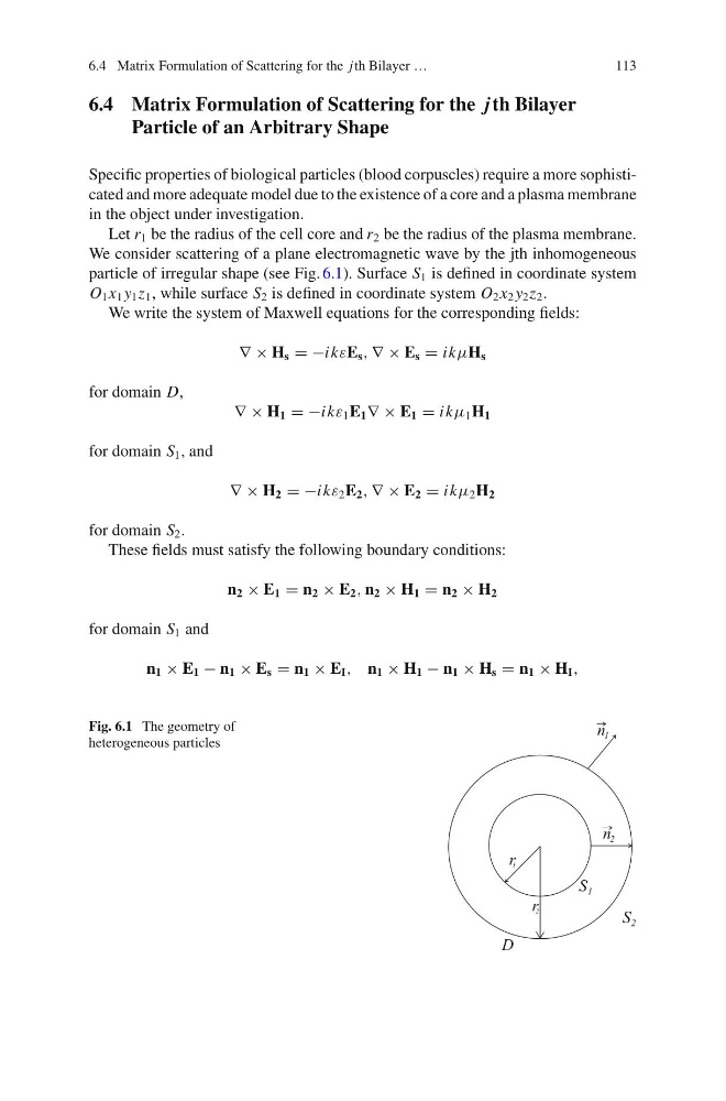
Specific properties of biological particles (blood corpuscles) require a more sophisticated and more adequate model due to the existence of a core and a plasma membrane
in the object under investigation.
Let r 1 be the radius of the cell core and r 2 be the radius of the plasma membrane.
We consider scattering of a plane electromagnetic wave by the jth inhomogeneous
particle of irregular shape (see Fig. 6.1). Surface S 1 is defined in coordinate system
O 1 x 1 y 1 z 1 , while surface S 2 is defined in coordinate system O 2 x 2 y 2 z 2 .
We write the system of Maxwell equations for the corresponding fields:
∇ × H s = −ikεE s , ∇ × E s = ikμH s
for domain D,
∇ × H 1 = −ikε 1 E 1 ∇ × E 1 = ikμ 1 H 1
for domain S 1 , and
∇ × H 2 = −ikε 2 E 2 , ∇ × E 2 = ikμ 2 H 2
for domain S 2 .
These fields must satisfy the following boundary conditions:
n 2 × E 1 = n 2 × E 2 , n 2 × H 1 = n 2 × H 2
for domain S 1 and
n 1 × E 1 − n 1 × E s = n 1 × E I , n 1 × H 1 − n 1 × H s = n 1 × H I ,
Fig. 6.1 The geometry of
heterogeneous particles
S 2
D
r
r
n 1
S 1
2
1
n 2
113
6.4 Matrix Formulation of Scattering for the j th Bilayer
Particle of an Arbitrary Shape
Specific properties of biological particles (blood corpuscles) require a more sophisticated and more adequate model due to the existence of a core and a plasma membrane
in the object under investigation.
Let r 1 be the radius of the cell core and r 2 be the radius of the plasma membrane.
We consider scattering of a plane electromagnetic wave by the jth inhomogeneous
particle of irregular shape (see Fig. 6.1). Surface S 1 is defined in coordinate system
O 1 x 1 y 1 z 1 , while surface S 2 is defined in coordinate system O 2 x 2 y 2 z 2 .
We write the system of Maxwell equations for the corresponding fields:
∇ × H s = −ikεE s , ∇ × E s = ikμH s
for domain D,
∇ × H 1 = −ikε 1 E 1 ∇ × E 1 = ikμ 1 H 1
for domain S 1 , and
∇ × H 2 = −ikε 2 E 2 , ∇ × E 2 = ikμ 2 H 2
for domain S 2 .
These fields must satisfy the following boundary conditions:
n 2 × E 1 = n 2 × E 2 , n 2 × H 1 = n 2 × H 2
for domain S 1 and
n 1 × E 1 − n 1 × E s = n 1 × E I , n 1 × H 1 − n 1 × H s = n 1 × H I ,
Fig. 6.1 The geometry of
heterogeneous particles
S 2
D
r
r
n 1
S 1
2
1
n 2