

5 EEG Source Imaging and Multimodal Neuroimaging
105
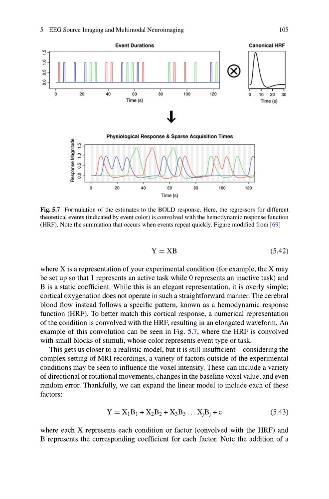
Fig. 5.7 Formulation of the estimates to the BOLD response. Here, the regressors for different
theoretical events (indicated by event color) is convolved with the hemodynamic response function
(HRF). Note the summation that occurs when events repeat quickly. Figure modified from [69]
Y XB
(5.42)
where X is a representation of your experimental condition (for example, the X may
be set up so that 1 represents an active task while 0 represents an inactive task) and
B is a static coefficient. While this is an elegant representation, it is overly simple;
cortical oxygenation does not operate in such a straightforward manner. The cerebral
blood flow instead follows a specific pattern, known as a hemodynamic response
function (HRF). To better match this cortical response, a numerical representation
of the condition is convolved with the HRF, resulting in an elongated waveform. An
example of this convolution can be seen in Fig. 5.7, where the HRF is convolved
with small blocks of stimuli, whose color represents event type or task.
This gets us closer to a realistic model, but it is still insufficient—considering the
complex setting of MRI recordings, a variety of factors outside of the experimental
conditions may be seen to influence the voxel intensity. These can include a variety
of directional or rotational movements, changes in the baseline voxel value, and even
random error. Thankfully, we can expand the linear model to include each of these
factors:
Y X 1 B 1 + X 2 B 2 + X 3 B 3 . . . X j B j + e
(5.43)
where each X represents each condition or factor (convolved with the HRF) and
B represents the corresponding coefficient for each factor. Note the addition of a
105
Fig. 5.7 Formulation of the estimates to the BOLD response. Here, the regressors for different
theoretical events (indicated by event color) is convolved with the hemodynamic response function
(HRF). Note the summation that occurs when events repeat quickly. Figure modified from [69]
Y XB
(5.42)
where X is a representation of your experimental condition (for example, the X may
be set up so that 1 represents an active task while 0 represents an inactive task) and
B is a static coefficient. While this is an elegant representation, it is overly simple;
cortical oxygenation does not operate in such a straightforward manner. The cerebral
blood flow instead follows a specific pattern, known as a hemodynamic response
function (HRF). To better match this cortical response, a numerical representation
of the condition is convolved with the HRF, resulting in an elongated waveform. An
example of this convolution can be seen in Fig. 5.7, where the HRF is convolved
with small blocks of stimuli, whose color represents event type or task.
This gets us closer to a realistic model, but it is still insufficient—considering the
complex setting of MRI recordings, a variety of factors outside of the experimental
conditions may be seen to influence the voxel intensity. These can include a variety
of directional or rotational movements, changes in the baseline voxel value, and even
random error. Thankfully, we can expand the linear model to include each of these
factors:
Y X 1 B 1 + X 2 B 2 + X 3 B 3 . . . X j B j + e
(5.43)
where each X represents each condition or factor (convolved with the HRF) and
B represents the corresponding coefficient for each factor. Note the addition of a