

model estimations, possibly due to (1) substantial and frequent variations of the
water table surface which generated drainage and imbibition, and de facto hysteresis
(trapping a substantial quantity of LNAPL); and/or (2) the residual saturations taken
into account in the model were too low.
Once the entire recoverable free product was pumped, the water pumps were
turned on intermittently to increase soil water flushing and reduce rebound effects.
The environmental impact was monitored throughout the treatment (quality of
groundwater and surface water was monitored, as was waste).
The groundwater still had high concentrations beneath and immediately downstream of the contamination source. This led to a cost–benefit analysis to assess the
acceptability of this residual contamination.
2.7.1.4 Cost–Benefit Analysis
The maximum acceptable concentrations immediately downstream of the site were
calculated so as not to have any impact on the drinking water supply well or the river
(i.e., concentrations below the standards for drinking water and surface water
resources). The quantity of hydrocarbons remaining in the dissolved phase immediately downstream of the residual pollution source has been determined through
iterations using Visual MODFLOW. The hydrodynamic parameters considered are
identical to those mentioned previously in Sect. 2.7.1.2. The hydro-dispersive
parameters used are displayed in Table 2.14. As a first approach, the parameters
were differentiated by TPH fraction.
As a first approach, and to be on the safe side, we considered the pollution source
as infinite. The results of hydrodynamic and hydro-dispersive modeling are shown in
Figs. 2.35, 2.36, 2.37, and 2.38.
The residual pollution should not generate downstream concentrations above the
maximum acceptable concentrations for the drinking water supply and river
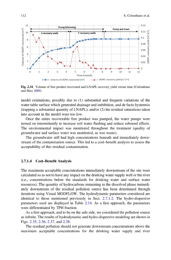
Fig. 2.34 Volume of free product recovered and LNAPL recovery yield versus time (Colombano
and Hiez 2009)
112
S. Colombano et al.
water table surface which generated drainage and imbibition, and de facto hysteresis
(trapping a substantial quantity of LNAPL); and/or (2) the residual saturations taken
into account in the model were too low.
Once the entire recoverable free product was pumped, the water pumps were
turned on intermittently to increase soil water flushing and reduce rebound effects.
The environmental impact was monitored throughout the treatment (quality of
groundwater and surface water was monitored, as was waste).
The groundwater still had high concentrations beneath and immediately downstream of the contamination source. This led to a cost–benefit analysis to assess the
acceptability of this residual contamination.
2.7.1.4 Cost–Benefit Analysis
The maximum acceptable concentrations immediately downstream of the site were
calculated so as not to have any impact on the drinking water supply well or the river
(i.e., concentrations below the standards for drinking water and surface water
resources). The quantity of hydrocarbons remaining in the dissolved phase immediately downstream of the residual pollution source has been determined through
iterations using Visual MODFLOW. The hydrodynamic parameters considered are
identical to those mentioned previously in Sect. 2.7.1.2. The hydro-dispersive
parameters used are displayed in Table 2.14. As a first approach, the parameters
were differentiated by TPH fraction.
As a first approach, and to be on the safe side, we considered the pollution source
as infinite. The results of hydrodynamic and hydro-dispersive modeling are shown in
Figs. 2.35, 2.36, 2.37, and 2.38.
The residual pollution should not generate downstream concentrations above the
maximum acceptable concentrations for the drinking water supply and river
Fig. 2.34 Volume of free product recovered and LNAPL recovery yield versus time (Colombano
and Hiez 2009)
112
S. Colombano et al.