

2.3.1 Global Scoring
Cross-Correlation
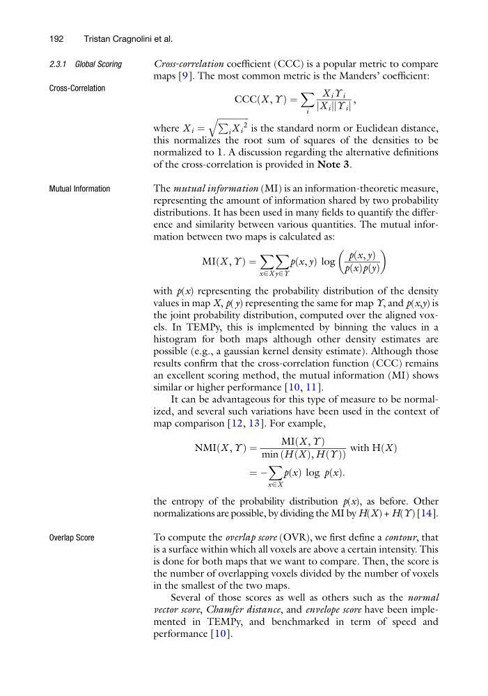
Cross-correlation coefficient (CCC) is a popular metric to compare
maps [9]. The most common metric is the Manders’ coefficient:
CCC X , Y
ð
Þ¼
X
i
X i Y i
X i
j j Y i
j j
,
where X i ¼
ffiffiffiffiffiffiffiffiffiffiffiffiffiffi ffi
P
i X i
2
q
is the standard norm or Euclidean distance,
this normalizes the root sum of squares of the densities to be
normalized to 1. A discussion regarding the alternative definitions
of the cross-correlation is provided in Note 3.
Mutual Information
The mutual information (MI) is an information-theoretic measure,
representing the amount of information shared by two probability
distributions. It has been used in many fields to quantify the difference and similarity between various quantities. The mutual information between two maps is calculated as:
MI X , Y
ð
Þ¼
X
x∈X
X
y∈Y
p x, y
ð Þ log
p x, y
ð Þ
p x
ð Þp y
ð Þ
with p(x) representing the probability distribution of the density
values in map X, p( y) representing the same for map Y, and p(x,y) is
the joint probability distribution, computed over the aligned voxels. In TEMPy, this is implemented by binning the values in a
histogram for both maps although other density estimates are
possible (e.g., a gaussian kernel density estimate). Although those
results confirm that the cross-correlation function (CCC) remains
an excellent scoring method, the mutual information (MI) shows
similar or higher performance [10, 11].
It can be advantageous for this type of measure to be normalized, and several such variations have been used in the context of
map comparison [12, 13]. For example,
NMI X , Y
ð
Þ¼
MI X , Y
ð
Þ
min H X
ð Þ, H Y
ð Þ
ð
Þ
with H X
ð Þ
¼ À
X
x∈X
p x
ð Þ log p x
ð Þ:
the entropy of the probability distribution p(x), as before. Other
normalizations are possible, by dividing the MI by H(X) + H(Y) [14].
Overlap Score
To compute the overlap score (OVR), we first define a contour, that
is a surface within which all voxels are above a certain intensity. This
is done for both maps that we want to compare. Then, the score is
the number of overlapping voxels divided by the number of voxels
in the smallest of the two maps.
Several of those scores as well as others such as the normal
vector score, Chamfer distance, and envelope score have been implemented in TEMPy, and benchmarked in term of speed and
performance [10].
192
Tristan Cragnolini et al.
Cross-Correlation
Cross-correlation coefficient (CCC) is a popular metric to compare
maps [9]. The most common metric is the Manders’ coefficient:
CCC X , Y
ð
Þ¼
X
i
X i Y i
X i
j j Y i
j j
,
where X i ¼
ffiffiffiffiffiffiffiffiffiffiffiffiffiffi ffi
P
i X i
2
q
is the standard norm or Euclidean distance,
this normalizes the root sum of squares of the densities to be
normalized to 1. A discussion regarding the alternative definitions
of the cross-correlation is provided in Note 3.
Mutual Information
The mutual information (MI) is an information-theoretic measure,
representing the amount of information shared by two probability
distributions. It has been used in many fields to quantify the difference and similarity between various quantities. The mutual information between two maps is calculated as:
MI X , Y
ð
Þ¼
X
x∈X
X
y∈Y
p x, y
ð Þ log
p x, y
ð Þ
p x
ð Þp y
ð Þ
with p(x) representing the probability distribution of the density
values in map X, p( y) representing the same for map Y, and p(x,y) is
the joint probability distribution, computed over the aligned voxels. In TEMPy, this is implemented by binning the values in a
histogram for both maps although other density estimates are
possible (e.g., a gaussian kernel density estimate). Although those
results confirm that the cross-correlation function (CCC) remains
an excellent scoring method, the mutual information (MI) shows
similar or higher performance [10, 11].
It can be advantageous for this type of measure to be normalized, and several such variations have been used in the context of
map comparison [12, 13]. For example,
NMI X , Y
ð
Þ¼
MI X , Y
ð
Þ
min H X
ð Þ, H Y
ð Þ
ð
Þ
with H X
ð Þ
¼ À
X
x∈X
p x
ð Þ log p x
ð Þ:
the entropy of the probability distribution p(x), as before. Other
normalizations are possible, by dividing the MI by H(X) + H(Y) [14].
Overlap Score
To compute the overlap score (OVR), we first define a contour, that
is a surface within which all voxels are above a certain intensity. This
is done for both maps that we want to compare. Then, the score is
the number of overlapping voxels divided by the number of voxels
in the smallest of the two maps.
Several of those scores as well as others such as the normal
vector score, Chamfer distance, and envelope score have been implemented in TEMPy, and benchmarked in term of speed and
performance [10].
192
Tristan Cragnolini et al.