

implementation to identify the shortest paths of communication
between two sites. Indeed, communication in PSN is expected to
work more efficiently through the shortest paths between two distal
sites [122]. The PSN analysis sheds light on the atomic details
behind the distal communication and also identifies the most
important components in the mechanism. In the p53 example, it
allowed identifying the residues in the N-terminal tail as important
in modulating the conformation of the S6-S7 loop together with
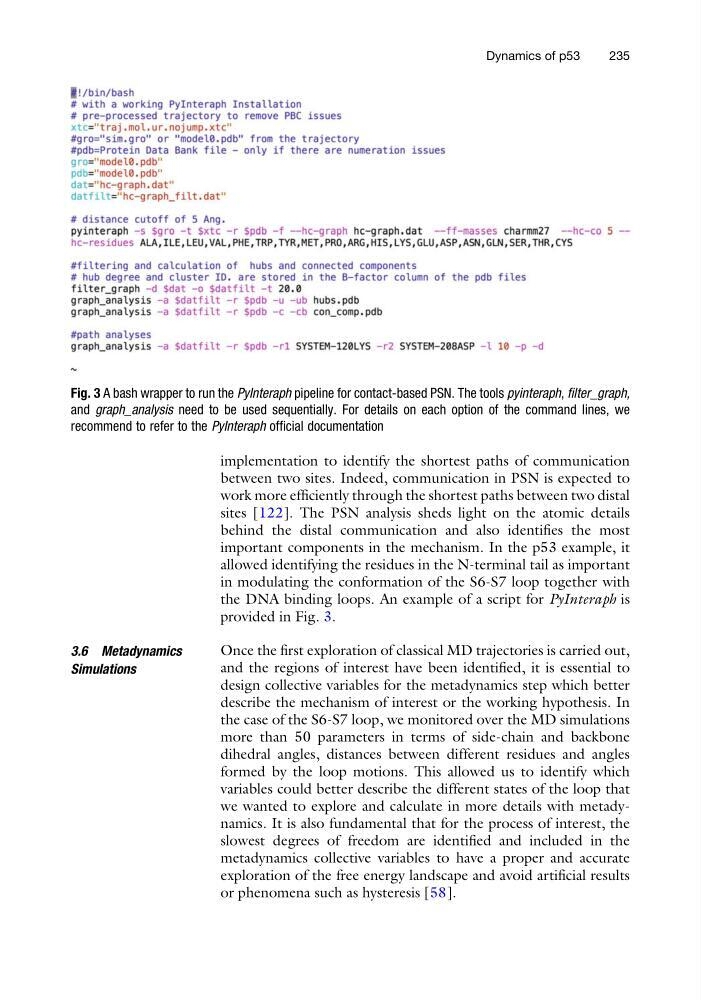
the DNA binding loops. An example of a script for PyInteraph is
provided in Fig. 3.
3.6 Metadynamics
Simulations
Once the first exploration of classical MD trajectories is carried out,
and the regions of interest have been identified, it is essential to
design collective variables for the metadynamics step which better
describe the mechanism of interest or the working hypothesis. In
the case of the S6-S7 loop, we monitored over the MD simulations
more than 50 parameters in terms of side-chain and backbone
dihedral angles, distances between different residues and angles
formed by the loop motions. This allowed us to identify which
variables could better describe the different states of the loop that
we wanted to explore and calculate in more details with metadynamics. It is also fundamental that for the process of interest, the
slowest degrees of freedom are identified and included in the
metadynamics collective variables to have a proper and accurate
exploration of the free energy landscape and avoid artificial results
or phenomena such as hysteresis [58].
Fig. 3 A bash wrapper to run the PyInteraph pipeline for contact-based PSN. The tools pyinteraph, filter_graph,
and graph_analysis need to be used sequentially. For details on each option of the command lines, we
recommend to refer to the PyInteraph official documentation
Dynamics of p53
235
between two sites. Indeed, communication in PSN is expected to
work more efficiently through the shortest paths between two distal
sites [122]. The PSN analysis sheds light on the atomic details
behind the distal communication and also identifies the most
important components in the mechanism. In the p53 example, it
allowed identifying the residues in the N-terminal tail as important
in modulating the conformation of the S6-S7 loop together with
the DNA binding loops. An example of a script for PyInteraph is
provided in Fig. 3.
3.6 Metadynamics
Simulations
Once the first exploration of classical MD trajectories is carried out,
and the regions of interest have been identified, it is essential to
design collective variables for the metadynamics step which better
describe the mechanism of interest or the working hypothesis. In
the case of the S6-S7 loop, we monitored over the MD simulations
more than 50 parameters in terms of side-chain and backbone
dihedral angles, distances between different residues and angles
formed by the loop motions. This allowed us to identify which
variables could better describe the different states of the loop that
we wanted to explore and calculate in more details with metadynamics. It is also fundamental that for the process of interest, the
slowest degrees of freedom are identified and included in the
metadynamics collective variables to have a proper and accurate
exploration of the free energy landscape and avoid artificial results
or phenomena such as hysteresis [58].
Fig. 3 A bash wrapper to run the PyInteraph pipeline for contact-based PSN. The tools pyinteraph, filter_graph,
and graph_analysis need to be used sequentially. For details on each option of the command lines, we
recommend to refer to the PyInteraph official documentation
Dynamics of p53
235