

432
when determining genetic diversity), our grain sizes span an even wider range, from
roughly 2 nm (in the case of the DNA double helix; van Holde 1989) to roughly
1 km (for “Pando,” a large clonal aspen stand (DeWoody et al. 2008), a range of
approximately 12 orders of magnitude). A rule of thumb for distinguishing spectral
differences is that the sampling grain size should be smaller than the cross-section
of the target (e.g., leaf or individual canopy crown in the case of individual plants;
Woodcock and Strahler 1987). These numbers imply that the sampling grain size
needs to span an extremely wide range to properly match all our definitions of biodiversity. Clearly, this is not possible from a single instrument, but can be considered in multi-scale field campaigns employing multiple instruments and platforms.
Additional challenges arise when designing a field campaign to validate remotely
sensed biodiversity data. Many field sampling methods for species richness entail
quadrat or transect sampling (Bonar et al. 2011), neither of which is well-matched
to the size, shape, and location of typical airborne or satellite pixels. Moreover, our
classical definitions of biodiversity at different scales (alpha, beta, or gamma) reflect
relative rather than absolute spatial scales and often poorly match the scale of both
field sampling and RS. These challenges of scale mismatch abound and require
careful attention to definitions and sampling protocols.
Similar issues of scale mismatch arise when exploring plant traits with RS. It
is unclear how well the ability to detect leaf traits transcends spatial scales, with
some studies suggesting certain leaf traits (nitrogen content) cannot be detected
at the sampling scale of a typical aircraft or satellite pixel (Knyazikhin et al.
2013). However, many leaf traits (if not all) can be detected at the canopy scale
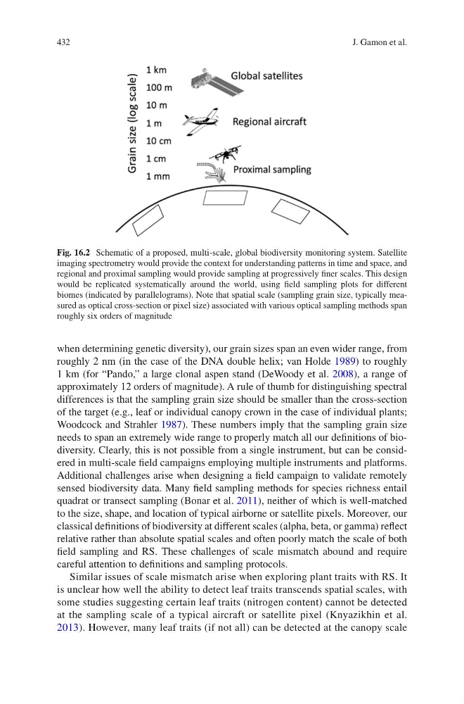
Fig. 16.2 Schematic of a proposed, multi-scale, global biodiversity monitoring system. Satellite
imaging spectrometry would provide the context for understanding patterns in time and space, and
regional and proximal sampling would provide sampling at progressively finer scales. This design
would be replicated systematically around the world, using field sampling plots for different
biomes (indicated by parallelograms). Note that spatial scale (sampling grain size, typically measured as optical cross-section or pixel size) associated with various optical sampling methods span
roughly six orders of magnitude
J. Gamon et al.
when determining genetic diversity), our grain sizes span an even wider range, from
roughly 2 nm (in the case of the DNA double helix; van Holde 1989) to roughly
1 km (for “Pando,” a large clonal aspen stand (DeWoody et al. 2008), a range of
approximately 12 orders of magnitude). A rule of thumb for distinguishing spectral
differences is that the sampling grain size should be smaller than the cross-section
of the target (e.g., leaf or individual canopy crown in the case of individual plants;
Woodcock and Strahler 1987). These numbers imply that the sampling grain size
needs to span an extremely wide range to properly match all our definitions of biodiversity. Clearly, this is not possible from a single instrument, but can be considered in multi-scale field campaigns employing multiple instruments and platforms.
Additional challenges arise when designing a field campaign to validate remotely
sensed biodiversity data. Many field sampling methods for species richness entail
quadrat or transect sampling (Bonar et al. 2011), neither of which is well-matched
to the size, shape, and location of typical airborne or satellite pixels. Moreover, our
classical definitions of biodiversity at different scales (alpha, beta, or gamma) reflect
relative rather than absolute spatial scales and often poorly match the scale of both
field sampling and RS. These challenges of scale mismatch abound and require
careful attention to definitions and sampling protocols.
Similar issues of scale mismatch arise when exploring plant traits with RS. It
is unclear how well the ability to detect leaf traits transcends spatial scales, with
some studies suggesting certain leaf traits (nitrogen content) cannot be detected
at the sampling scale of a typical aircraft or satellite pixel (Knyazikhin et al.
2013). However, many leaf traits (if not all) can be detected at the canopy scale
Fig. 16.2 Schematic of a proposed, multi-scale, global biodiversity monitoring system. Satellite
imaging spectrometry would provide the context for understanding patterns in time and space, and
regional and proximal sampling would provide sampling at progressively finer scales. This design
would be replicated systematically around the world, using field sampling plots for different
biomes (indicated by parallelograms). Note that spatial scale (sampling grain size, typically measured as optical cross-section or pixel size) associated with various optical sampling methods span
roughly six orders of magnitude
J. Gamon et al.