

218
Chap. 12; Meireles et al., Chap. 7), reducing the complexity of species identification
algorithms. For example, imaging spectroscopy allows mapping of functional traits,
by estimating vegetation traits for each pixel in an image (Wang et al. 2019; Asner
et al. 2017; Martin, Chap. 5). Plant spectra obtained from imaging spectroscopy at
different spatial resolutions can in turn be used to detect different aspects and
traits—within- and between-species differences in morphology, foliar chemistry,
life history strategies—of plant species (Ustin and Gamon 2010; Cavender- Bares
et al. 2017; Schweiger et al. 2018) and the correct identification of different taxonomic levels from populations to species to clades (Cavender-Bares et al. 2016).
Thus, the integration of spectral approaches with techniques for modeling species
ecological niches has the potential to produce reliable information of species distributions and co-occurrence, filling current gaps about species-environment relationships at a range of spatial scales and levels of organization—from species to
communities—increasing the accuracy of direct detection assignments, and enabling
monitoring of changes in biodiversity, one of the premises for the sustainable management of the biosphere (Pinto-Ledezma and Rivero 2014; Fernández et al.,
Chap. 18).
Acknowledgments We thank Julián Velasco for his advice with ENM/SDM analyses. J.N.P-L.
was supported by the University of Minnesota College of Biological Sciences’ Grand Challenges
in Biology Postdoctoral Program. We acknowledge the bioDISCOVERY community at the
University of Zürich for important discussions and the NSF Research Coordination Network
“Biodiversity Across Scales.”
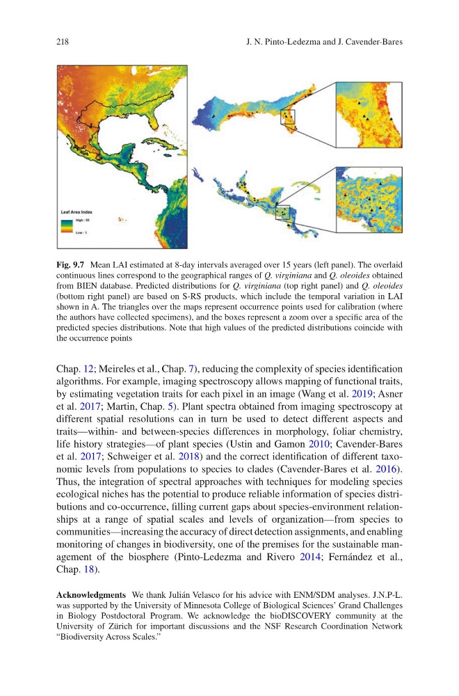
Fig. 9.7 Mean LAI estimated at 8-day intervals averaged over 15 years (left panel). The overlaid
continuous lines correspond to the geographical ranges of Q. virginiana and Q. oleoides obtained
from BIEN database. Predicted distributions for Q. virginiana (top right panel) and Q. oleoides
(bottom right panel) are based on S-RS products, which include the temporal variation in LAI
shown in A. The triangles over the maps represent occurrence points used for calibration (where
the authors have collected specimens), and the boxes represent a zoom over a specific area of the
predicted species distributions. Note that high values of the predicted distributions coincide with
the occurrence points
J. N. Pinto-Ledezma and J. Cavender-Bares
Chap. 12; Meireles et al., Chap. 7), reducing the complexity of species identification
algorithms. For example, imaging spectroscopy allows mapping of functional traits,
by estimating vegetation traits for each pixel in an image (Wang et al. 2019; Asner
et al. 2017; Martin, Chap. 5). Plant spectra obtained from imaging spectroscopy at
different spatial resolutions can in turn be used to detect different aspects and
traits—within- and between-species differences in morphology, foliar chemistry,
life history strategies—of plant species (Ustin and Gamon 2010; Cavender- Bares
et al. 2017; Schweiger et al. 2018) and the correct identification of different taxonomic levels from populations to species to clades (Cavender-Bares et al. 2016).
Thus, the integration of spectral approaches with techniques for modeling species
ecological niches has the potential to produce reliable information of species distributions and co-occurrence, filling current gaps about species-environment relationships at a range of spatial scales and levels of organization—from species to
communities—increasing the accuracy of direct detection assignments, and enabling
monitoring of changes in biodiversity, one of the premises for the sustainable management of the biosphere (Pinto-Ledezma and Rivero 2014; Fernández et al.,
Chap. 18).
Acknowledgments We thank Julián Velasco for his advice with ENM/SDM analyses. J.N.P-L.
was supported by the University of Minnesota College of Biological Sciences’ Grand Challenges
in Biology Postdoctoral Program. We acknowledge the bioDISCOVERY community at the
University of Zürich for important discussions and the NSF Research Coordination Network
“Biodiversity Across Scales.”
Fig. 9.7 Mean LAI estimated at 8-day intervals averaged over 15 years (left panel). The overlaid
continuous lines correspond to the geographical ranges of Q. virginiana and Q. oleoides obtained
from BIEN database. Predicted distributions for Q. virginiana (top right panel) and Q. oleoides
(bottom right panel) are based on S-RS products, which include the temporal variation in LAI
shown in A. The triangles over the maps represent occurrence points used for calibration (where
the authors have collected specimens), and the boxes represent a zoom over a specific area of the
predicted species distributions. Note that high values of the predicted distributions coincide with
the occurrence points
J. N. Pinto-Ledezma and J. Cavender-Bares