

214
9.4 Perspectives
The field of ecological niche and species distribution modeling contributes significantly to our capacity to evaluate and describe the effect of geographical and environmental features on species distributions and has become in one of the most
widely applied tools for the assessment of the impact of climate change and human
activities on species and communities, biological invasions, epidemiology, and conservation biology (Peterson et al. 2011; Guisan et al. 2017). However, despite
important advances in theory (Soberón 2007; Colwell and Rangel 2009; Soberón
and Nakamura 2009; Peterson et al. 2011), methods, and algorithms (reviewed in
Duarte et al. 2019; see also Warren et al. 2018) and practical applications (GuilleraArroita et al. 2015; Cord et al. 2017; Sanín and Anderson 2018), most studies still
rely on the use of interpolated climate data as environmental predictors (Saatchi
et al. 2008; Waltari et al. 2014). In this article we compare the performance of environmental data derived from interpolated climate surfaces data (i.e., WorldClim)
and S-RS products data (i.e., LAI and NDVI). Specifically, using live oaks as a case
study, we show the advances and potential caveats in using S-RS data in describing
and predicting species-environment relationships. Overall, our analyses show that
S-RS products perform, as well as products from interpolated climate surfaces as
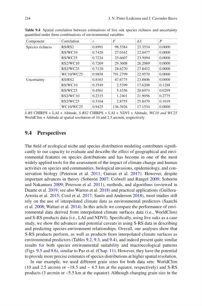
environmental predictors (Tables 9.2, 9.3, and 9.4), and indeed present quite similar
results for both species environmental suitability and macroecological patterns
(Figs. 9.5 and 9.6), similar to Paz et al. (Chap. 11). However, they have the potential
to provide more precise estimates of species distributions at higher spatial resolution.
In our example, we used different grain sizes for both data sets: WorldClim
(10 and 2.5 arcmin or ~18.5 and ~ 4.5 km at the equator, respectively) and S-RS
products (3 arcmin or ~5.5 km at the equator). Although changing grain size in the
Table 9.4 Spatial correlation between estimations of live oak species richness and uncertainty
quantified under three combinations of environmental variables
Component
Correlation
r
F
d.f.
P
Species richness
RS/RS2
0.8991
98.5384
23.3534
0.0000
RS/WC10
0.7420
27.0162
22.0477
0.0000
RS/WC25
0.7224
25.6607
23.5094
0.0000
RS2/WC10
0.7269
29.3608
26.2069
0.0000
RS2/WC25
0.7120
28.6270
27.8452
0.0000
WC10/WC25
0.9858
791.2799
22.9570
0.0000
Uncertainty
RS/RS2
0.8163
47.6775
23.8806
0.0000
RS/WC10
0.3549
2.5399
17.6208
0.1288
RS/WC25
0.4561
5.4356
20.6974
0.0299
RS2/WC10
0.2315
1.2401
21.9056
0.2775
RS2/WC25
0.3164
2.8755
25.8479
0.1019
WC10/WC25
0.9425
136.3926
17.1534
0.0000
S-RS CHIRPS + LAI + Altitude, S-RS2 CHIRPS + LAI + NDVI + Altitude, WC10 and WC25
WorldClim + Altitude at spatial resolution of 10 and 2.5 arcmin, respectively
J. N. Pinto-Ledezma and J. Cavender-Bares
9.4 Perspectives
The field of ecological niche and species distribution modeling contributes significantly to our capacity to evaluate and describe the effect of geographical and environmental features on species distributions and has become in one of the most
widely applied tools for the assessment of the impact of climate change and human
activities on species and communities, biological invasions, epidemiology, and conservation biology (Peterson et al. 2011; Guisan et al. 2017). However, despite
important advances in theory (Soberón 2007; Colwell and Rangel 2009; Soberón
and Nakamura 2009; Peterson et al. 2011), methods, and algorithms (reviewed in
Duarte et al. 2019; see also Warren et al. 2018) and practical applications (GuilleraArroita et al. 2015; Cord et al. 2017; Sanín and Anderson 2018), most studies still
rely on the use of interpolated climate data as environmental predictors (Saatchi
et al. 2008; Waltari et al. 2014). In this article we compare the performance of environmental data derived from interpolated climate surfaces data (i.e., WorldClim)
and S-RS products data (i.e., LAI and NDVI). Specifically, using live oaks as a case
study, we show the advances and potential caveats in using S-RS data in describing
and predicting species-environment relationships. Overall, our analyses show that
S-RS products perform, as well as products from interpolated climate surfaces as
environmental predictors (Tables 9.2, 9.3, and 9.4), and indeed present quite similar
results for both species environmental suitability and macroecological patterns
(Figs. 9.5 and 9.6), similar to Paz et al. (Chap. 11). However, they have the potential
to provide more precise estimates of species distributions at higher spatial resolution.
In our example, we used different grain sizes for both data sets: WorldClim
(10 and 2.5 arcmin or ~18.5 and ~ 4.5 km at the equator, respectively) and S-RS
products (3 arcmin or ~5.5 km at the equator). Although changing grain size in the
Table 9.4 Spatial correlation between estimations of live oak species richness and uncertainty
quantified under three combinations of environmental variables
Component
Correlation
r
F
d.f.
P
Species richness
RS/RS2
0.8991
98.5384
23.3534
0.0000
RS/WC10
0.7420
27.0162
22.0477
0.0000
RS/WC25
0.7224
25.6607
23.5094
0.0000
RS2/WC10
0.7269
29.3608
26.2069
0.0000
RS2/WC25
0.7120
28.6270
27.8452
0.0000
WC10/WC25
0.9858
791.2799
22.9570
0.0000
Uncertainty
RS/RS2
0.8163
47.6775
23.8806
0.0000
RS/WC10
0.3549
2.5399
17.6208
0.1288
RS/WC25
0.4561
5.4356
20.6974
0.0299
RS2/WC10
0.2315
1.2401
21.9056
0.2775
RS2/WC25
0.3164
2.8755
25.8479
0.1019
WC10/WC25
0.9425
136.3926
17.1534
0.0000
S-RS CHIRPS + LAI + Altitude, S-RS2 CHIRPS + LAI + NDVI + Altitude, WC10 and WC25
WorldClim + Altitude at spatial resolution of 10 and 2.5 arcmin, respectively
J. N. Pinto-Ledezma and J. Cavender-Bares