

20
V. Blazek
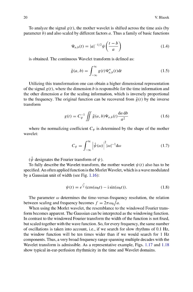
To analyze the signal g(t), the mother wavelet is shifted across the time axis (by
parameter b) and also scaled by different factors a. Thus a family of basic functions
a,b (t) = |a|
−1/2
ψ
t − b
a
(1.4)
is obtained. The continuous Wavelet transform is defined as:
˜
g(a, b) =
∞
−∞
g(t))
∗
a,b (t)dt
(1.5)
Utilizing this transformation one can obtain a higher dimensional representation
of the signal g(t), where the dimension b is responsible for the time information and
the other dimension a for the scaling information, which is inversely proportional
to the frequency. The original function can be recovered from ˜
g(t) by the inverse
transform
g(t) = C
−1
ψ
¨
˜
g(a, b)) a,b (t)
da db
a 2
(1.6)
where the normalizing coefficient C ψ is determined by the shape of the mother
wavelet:
C ψ =
∞
−∞
ˆ
ψ(ω)
2 |ω|
−1 dω
(1.7)
( ˆ
ψ designates the Fourier transform of ψ).
To fully describe the Wavelet transform, the mother wavelet ψ(t) also has to be
specified. An often applied function is the Morlet Wavelet, which is a wave modulated
by a Gaussian unit of width (see Fig. 1.16):
ψ(t) = e
t 2
2 (cos(ω 0 t) − i sin(ω 0 t)).
(1.8)
The parameter ω determines the time-versus-frequency resolution, the relation
between scaling and frequency becomes f = 2πω 0
a.
When using the Morlet wavelet, the resemblance to the windowed Fourier transform becomes apparent. The Gaussian can be interpreted as the windowing function.
In contrast to the windowed Fourier transform the width of the function is not fixed,
but scaled together with the wave function. So, for every frequency, the same number
of oscillations is taken into account, i.e., if we search for slow rhythms of 0.1 Hz,
the window function will be ten times wider than if we would search for 1 Hz
components. Thus, a very broad frequency range spanning multiple decades with the
Wavelet transform is admissible. As a representative example, Figs. 1.17 and 1.18
show typical in-ear-perfusion rhythmicity in the time and Wavelet domains.
V. Blazek
To analyze the signal g(t), the mother wavelet is shifted across the time axis (by
parameter b) and also scaled by different factors a. Thus a family of basic functions
a,b (t) = |a|
−1/2
ψ
t − b
a
(1.4)
is obtained. The continuous Wavelet transform is defined as:
˜
g(a, b) =
∞
−∞
g(t))
∗
a,b (t)dt
(1.5)
Utilizing this transformation one can obtain a higher dimensional representation
of the signal g(t), where the dimension b is responsible for the time information and
the other dimension a for the scaling information, which is inversely proportional
to the frequency. The original function can be recovered from ˜
g(t) by the inverse
transform
g(t) = C
−1
ψ
¨
˜
g(a, b)) a,b (t)
da db
a 2
(1.6)
where the normalizing coefficient C ψ is determined by the shape of the mother
wavelet:
C ψ =
∞
−∞
ˆ
ψ(ω)
2 |ω|
−1 dω
(1.7)
( ˆ
ψ designates the Fourier transform of ψ).
To fully describe the Wavelet transform, the mother wavelet ψ(t) also has to be
specified. An often applied function is the Morlet Wavelet, which is a wave modulated
by a Gaussian unit of width (see Fig. 1.16):
ψ(t) = e
t 2
2 (cos(ω 0 t) − i sin(ω 0 t)).
(1.8)
The parameter ω determines the time-versus-frequency resolution, the relation
between scaling and frequency becomes f = 2πω 0
a.
When using the Morlet wavelet, the resemblance to the windowed Fourier transform becomes apparent. The Gaussian can be interpreted as the windowing function.
In contrast to the windowed Fourier transform the width of the function is not fixed,
but scaled together with the wave function. So, for every frequency, the same number
of oscillations is taken into account, i.e., if we search for slow rhythms of 0.1 Hz,
the window function will be ten times wider than if we would search for 1 Hz
components. Thus, a very broad frequency range spanning multiple decades with the
Wavelet transform is admissible. As a representative example, Figs. 1.17 and 1.18
show typical in-ear-perfusion rhythmicity in the time and Wavelet domains.