

6 Identity by Descent in the Mapping of Genetic Traits
133
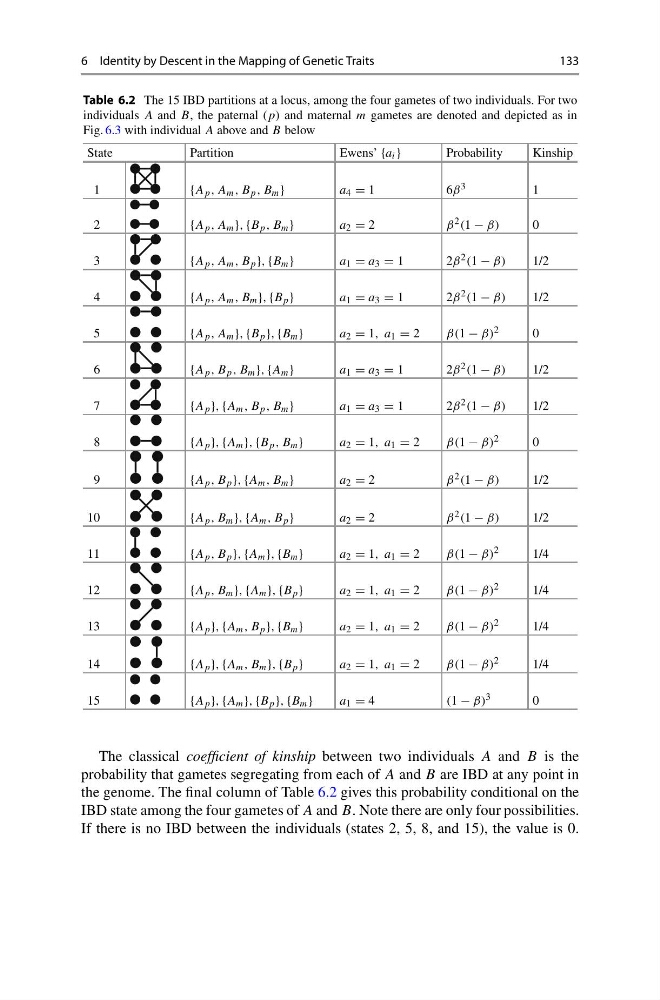
Table 6.2 The 15 IBD partitions at a locus, among the four gametes of two individuals. For two
individuals A and B, the paternal (p) and maternal m gametes are denoted and depicted as in
Fig. 6.3 with individual A above and B below
State
Partition
Ewens’ {a i }
Probability
Kinship
1
{A p , A m , B p , B m }
a 4 = 1
6β 3
1
2
{A p , A m }, {B p , B m }
a 2 = 2
β 2 (1 − β)
0
3
{A p , A m , B p }, {B m }
a 1 = a 3 = 1
2β 2 (1 − β)
1/2
4
{A p , A m , B m }, {B p }
a 1 = a 3 = 1
2β 2 (1 − β)
1/2
5
{A p , A m }, {B p }, {B m }
a 2 = 1, a 1 = 2
β(1 − β) 2
0
6
{A p , B p , B m }, {A m }
a 1 = a 3 = 1
2β 2 (1 − β)
1/2
7
{A p }, {A m , B p , B m }
a 1 = a 3 = 1
2β 2 (1 − β)
1/2
8
{A p }, {A m }, {B p , B m }
a 2 = 1, a 1 = 2
β(1 − β) 2
0
9
{A p , B p }, {A m , B m }
a 2 = 2
β 2 (1 − β)
1/2
10
{A p , B m }, {A m , B p }
a 2 = 2
β 2 (1 − β)
1/2
11
{A p , B p }, {A m }, {B m }
a 2 = 1, a 1 = 2
β(1 − β) 2
1/4
12
{A p , B m }, {A m }, {B p }
a 2 = 1, a 1 = 2
β(1 − β) 2
1/4
13
{A p }, {A m , B p }, {B m }
a 2 = 1, a 1 = 2
β(1 − β) 2
1/4
14
{A p }, {A m , B m }, {B p }
a 2 = 1, a 1 = 2
β(1 − β) 2
1/4
15
{A p }, {A m }, {B p }, {B m }
a 1 = 4
(1 − β) 3
0
The classical coefficient of kinship between two individuals A and B is the
probability that gametes segregating from each of A and B are IBD at any point in
the genome. The final column of Table 6.2 gives this probability conditional on the
IBD state among the four gametes of A and B. Note there are only four possibilities.
If there is no IBD between the individuals (states 2, 5, 8, and 15), the value is 0.
133
Table 6.2 The 15 IBD partitions at a locus, among the four gametes of two individuals. For two
individuals A and B, the paternal (p) and maternal m gametes are denoted and depicted as in
Fig. 6.3 with individual A above and B below
State
Partition
Ewens’ {a i }
Probability
Kinship
1
{A p , A m , B p , B m }
a 4 = 1
6β 3
1
2
{A p , A m }, {B p , B m }
a 2 = 2
β 2 (1 − β)
0
3
{A p , A m , B p }, {B m }
a 1 = a 3 = 1
2β 2 (1 − β)
1/2
4
{A p , A m , B m }, {B p }
a 1 = a 3 = 1
2β 2 (1 − β)
1/2
5
{A p , A m }, {B p }, {B m }
a 2 = 1, a 1 = 2
β(1 − β) 2
0
6
{A p , B p , B m }, {A m }
a 1 = a 3 = 1
2β 2 (1 − β)
1/2
7
{A p }, {A m , B p , B m }
a 1 = a 3 = 1
2β 2 (1 − β)
1/2
8
{A p }, {A m }, {B p , B m }
a 2 = 1, a 1 = 2
β(1 − β) 2
0
9
{A p , B p }, {A m , B m }
a 2 = 2
β 2 (1 − β)
1/2
10
{A p , B m }, {A m , B p }
a 2 = 2
β 2 (1 − β)
1/2
11
{A p , B p }, {A m }, {B m }
a 2 = 1, a 1 = 2
β(1 − β) 2
1/4
12
{A p , B m }, {A m }, {B p }
a 2 = 1, a 1 = 2
β(1 − β) 2
1/4
13
{A p }, {A m , B p }, {B m }
a 2 = 1, a 1 = 2
β(1 − β) 2
1/4
14
{A p }, {A m , B m }, {B p }
a 2 = 1, a 1 = 2
β(1 − β) 2
1/4
15
{A p }, {A m }, {B p }, {B m }
a 1 = 4
(1 − β) 3
0
The classical coefficient of kinship between two individuals A and B is the
probability that gametes segregating from each of A and B are IBD at any point in
the genome. The final column of Table 6.2 gives this probability conditional on the
IBD state among the four gametes of A and B. Note there are only four possibilities.
If there is no IBD between the individuals (states 2, 5, 8, and 15), the value is 0.