

241
Appendix
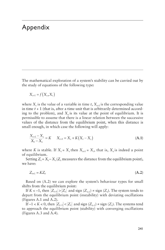
The mathematical exploration of a system’s stability can be carried out by
the study of equations of the following type:
X
f X X
t
s
t
+ = (
)
1
,
where X t is the value of a variable in time t, X t+1 is the corresponding value
in time t + 1 (that is, after a time unit that is arbitrarily determined according to the problem), and X s is its value at the point of equilibrium. It is
permissible to assume that there is a linear relation between the successive
values of the distance from the equilibrium point, when this distance is
small enough, in which case the following will apply:
X
X
X X
K X
X K X X
t
s
t
s
t
s
t
s
+
+
−
−
=
=
+
−
(
)
1
1
(a.1)
where K is stable. If X t = X s then X t+1 = X t , that is, X s is indeed a point
of equilibrium.
Setting Z t = X t – X s (Z t measures the distance from the equilibrium point),
we have:
Z
KZ
t
t
+ =
1
(a.2)
Based on (A.2) we can explore the system’s behaviour types for small
shifts from the equilibrium point:
If K < –1, then Z
Z
t
t
+ >
1
and sign (Z t+1 ) ≠ sign (Z t ). The system tends to
depart from the equilibrium point (instability) with deviating oscillations
(Figures A.1 and A.2).
If –1 < K < 0, then Z
Z
t
t
+ <
1
and sign (Z t+1 ) ≠ sign (Z t ). The systems tend
to approach the equilibrium point (stability) with converging oscillations
(Figures A.3 and A.4).
Appendix
The mathematical exploration of a system’s stability can be carried out by
the study of equations of the following type:
X
f X X
t
s
t
+ = (
)
1
,
where X t is the value of a variable in time t, X t+1 is the corresponding value
in time t + 1 (that is, after a time unit that is arbitrarily determined according to the problem), and X s is its value at the point of equilibrium. It is
permissible to assume that there is a linear relation between the successive
values of the distance from the equilibrium point, when this distance is
small enough, in which case the following will apply:
X
X
X X
K X
X K X X
t
s
t
s
t
s
t
s
+
+
−
−
=
=
+
−
(
)
1
1
(a.1)
where K is stable. If X t = X s then X t+1 = X t , that is, X s is indeed a point
of equilibrium.
Setting Z t = X t – X s (Z t measures the distance from the equilibrium point),
we have:
Z
KZ
t
t
+ =
1
(a.2)
Based on (A.2) we can explore the system’s behaviour types for small
shifts from the equilibrium point:
If K < –1, then Z
Z
t
t
+ >
1
and sign (Z t+1 ) ≠ sign (Z t ). The system tends to
depart from the equilibrium point (instability) with deviating oscillations
(Figures A.1 and A.2).
If –1 < K < 0, then Z
Z
t
t
+ <
1
and sign (Z t+1 ) ≠ sign (Z t ). The systems tend
to approach the equilibrium point (stability) with converging oscillations
(Figures A.3 and A.4).