

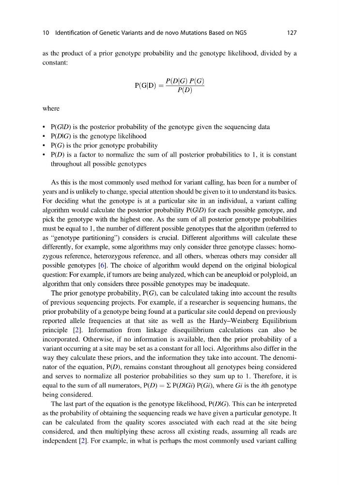
as the product of a prior genotype probability and the genotype likelihood, divided by a
constant:
P GjD
ð
Þ ¼
P DjG
ð
ÞP G
ð Þ
P D
ð Þ
where
• P(G|D) is the posterior probability of the genotype given the sequencing data
• P(D|G) is the genotype likelihood
• P(G) is the prior genotype probability
• P(D) is a factor to normalize the sum of all posterior probabilities to 1, it is constant
throughout all possible genotypes
As this is the most commonly used method for variant calling, has been for a number of
years and is unlikely to change, special attention should be given to it to understand its basics.
For deciding what the genotype is at a particular site in an individual, a variant calling
algorithm would calculate the posterior probability P(G|D) for each possible genotype, and
pick the genotype with the highest one. As the sum of all posterior genotype probabilities
must be equal to 1, the number of different possible genotypes that the algorithm (referred to
as “genotype partitioning”) considers is crucial. Different algorithms will calculate these
differently, for example, some algorithms may only consider three genotype classes: homozygous reference, heterozygous reference, and all others, whereas others may consider all
possible genotypes [6]. The choice of algorithm would depend on the original biological
question: For example, if tumors are being analyzed, which can be aneuploid or polyploid, an
algorithm that only considers three possible genotypes may be inadequate.
The prior genotype probability, P(G), can be calculated taking into account the results
of previous sequencing projects. For example, if a researcher is sequencing humans, the
prior probability of a genotype being found at a particular site could depend on previously
reported allele frequencies at that site as well as the Hardy–Weinberg Equilibrium
principle [2]. Information from linkage disequilibrium calculations can also be
incorporated. Otherwise, if no information is available, then the prior probability of a
variant occurring at a site may be set as a constant for all loci. Algorithms also differ in the
way they calculate these priors, and the information they take into account. The denominator of the equation, P(D), remains constant throughout all genotypes being considered
and serves to normalize all posterior probabilities so they sum up to 1. Therefore, it is
equal to the sum of all numerators, P(D) ¼ Σ P(D|Gi) P(Gi), where Gi is the ith genotype
being considered.
The last part of the equation is the genotype likelihood, P(D|G). This can be interpreted
as the probability of obtaining the sequencing reads we have given a particular genotype. It
can be calculated from the quality scores associated with each read at the site being
considered, and then multiplying these across all existing reads, assuming all reads are
independent [2]. For example, in what is perhaps the most commonly used variant calling
10 Identification of Genetic Variants and de novo Mutations Based on NGS
127
constant:
P GjD
ð
Þ ¼
P DjG
ð
ÞP G
ð Þ
P D
ð Þ
where
• P(G|D) is the posterior probability of the genotype given the sequencing data
• P(D|G) is the genotype likelihood
• P(G) is the prior genotype probability
• P(D) is a factor to normalize the sum of all posterior probabilities to 1, it is constant
throughout all possible genotypes
As this is the most commonly used method for variant calling, has been for a number of
years and is unlikely to change, special attention should be given to it to understand its basics.
For deciding what the genotype is at a particular site in an individual, a variant calling
algorithm would calculate the posterior probability P(G|D) for each possible genotype, and
pick the genotype with the highest one. As the sum of all posterior genotype probabilities
must be equal to 1, the number of different possible genotypes that the algorithm (referred to
as “genotype partitioning”) considers is crucial. Different algorithms will calculate these
differently, for example, some algorithms may only consider three genotype classes: homozygous reference, heterozygous reference, and all others, whereas others may consider all
possible genotypes [6]. The choice of algorithm would depend on the original biological
question: For example, if tumors are being analyzed, which can be aneuploid or polyploid, an
algorithm that only considers three possible genotypes may be inadequate.
The prior genotype probability, P(G), can be calculated taking into account the results
of previous sequencing projects. For example, if a researcher is sequencing humans, the
prior probability of a genotype being found at a particular site could depend on previously
reported allele frequencies at that site as well as the Hardy–Weinberg Equilibrium
principle [2]. Information from linkage disequilibrium calculations can also be
incorporated. Otherwise, if no information is available, then the prior probability of a
variant occurring at a site may be set as a constant for all loci. Algorithms also differ in the
way they calculate these priors, and the information they take into account. The denominator of the equation, P(D), remains constant throughout all genotypes being considered
and serves to normalize all posterior probabilities so they sum up to 1. Therefore, it is
equal to the sum of all numerators, P(D) ¼ Σ P(D|Gi) P(Gi), where Gi is the ith genotype
being considered.
The last part of the equation is the genotype likelihood, P(D|G). This can be interpreted
as the probability of obtaining the sequencing reads we have given a particular genotype. It
can be calculated from the quality scores associated with each read at the site being
considered, and then multiplying these across all existing reads, assuming all reads are
independent [2]. For example, in what is perhaps the most commonly used variant calling
10 Identification of Genetic Variants and de novo Mutations Based on NGS
127