

9.2.2 Local Alignment (Smith–Waterman Algorithm)
Local alignment performed by the Smith–Waterman algorithm [7] aims to determine
similarities between two nucleic acid or protein sequences. The main difference to the
global alignment is that negative scoring matrix cells are set to zero (Fig. 9.5).
For a better understanding of local/sub-regions alignment imagine you have a little Toy
genome (16 bp): CATGGTCATTGGTTCC.
Local alignment is a hash-based algorithm with two major approaches: hashing the
reference and the Burrows–Wheeler transform [8, 9]. The first step is to hash/index the
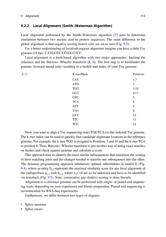
genome (forward strand only) resulting in a hash/k-mer index of your Toy genome:
k¼3
K-mer/Hash
Positions
CAT
1,7
ATG
2
TGG
3,10
GGT
4,11
GTC
5
TCA
6
ATT
8
TTG
9
GTT
12
TTC
13
TCC
14
Now, you want to align a Toy sequencing read (TGGTCA) to this indexed Toy genome.
The k-mer index can be used to quickly find candidate alignment locations in the reference
genome. For example, the k-mer TGG is assigned to Positions 3 and 10 and the k-mer TCA
to position 6. Thus, Burrows–Wheeler transform is just another way of doing exact matches
on hashes and check against genome and calculate a score.
This approach tries to identify the most similar subsequences that maximize the scoring
of their matching parts and the changes needed to transfer one subsequence into the other.
The dynamic programming approach tabularizes optimal subsolutions in matrix E (Fig.
9.4), where an entry E i,j represents the maximal similarity score for any local alignment of
the (sub)prefixes a x..i with b y..j , where x,y>0 are so far unknown and have to be identified
via traceback (Fig. 9.5). Note: consecutive gap (Indels) scoring is done linearly.
Alignment to a reference genome can be performed with single- or paired-end sequencing reads, depending on your experiment and library preparation. Paired-end sequencing is
recommended for RNA-Seq experiments.
Furthermore, we differ between two types of aligners:
• Splice unaware
• Splice aware
9 Alignment
115
Local alignment performed by the Smith–Waterman algorithm [7] aims to determine
similarities between two nucleic acid or protein sequences. The main difference to the
global alignment is that negative scoring matrix cells are set to zero (Fig. 9.5).
For a better understanding of local/sub-regions alignment imagine you have a little Toy
genome (16 bp): CATGGTCATTGGTTCC.
Local alignment is a hash-based algorithm with two major approaches: hashing the
reference and the Burrows–Wheeler transform [8, 9]. The first step is to hash/index the
genome (forward strand only) resulting in a hash/k-mer index of your Toy genome:
k¼3
K-mer/Hash
Positions
CAT
1,7
ATG
2
TGG
3,10
GGT
4,11
GTC
5
TCA
6
ATT
8
TTG
9
GTT
12
TTC
13
TCC
14
Now, you want to align a Toy sequencing read (TGGTCA) to this indexed Toy genome.
The k-mer index can be used to quickly find candidate alignment locations in the reference
genome. For example, the k-mer TGG is assigned to Positions 3 and 10 and the k-mer TCA
to position 6. Thus, Burrows–Wheeler transform is just another way of doing exact matches
on hashes and check against genome and calculate a score.
This approach tries to identify the most similar subsequences that maximize the scoring
of their matching parts and the changes needed to transfer one subsequence into the other.
The dynamic programming approach tabularizes optimal subsolutions in matrix E (Fig.
9.4), where an entry E i,j represents the maximal similarity score for any local alignment of
the (sub)prefixes a x..i with b y..j , where x,y>0 are so far unknown and have to be identified
via traceback (Fig. 9.5). Note: consecutive gap (Indels) scoring is done linearly.
Alignment to a reference genome can be performed with single- or paired-end sequencing reads, depending on your experiment and library preparation. Paired-end sequencing is
recommended for RNA-Seq experiments.
Furthermore, we differ between two types of aligners:
• Splice unaware
• Splice aware
9 Alignment
115