

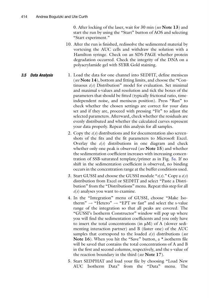
0. After locking of the laser, wait for 30 min (see Note 13) and
start the run by using the “Start” button of AOS and selecting
“Start experiment.”
10. After the run is finished, redissolve the sedimented material by
vortexing the AUC cells and withdraw the solution with a
Hamilton syringe. Check on an SDS-PAGE whether protein
degradation occurred. Check the integrity of the DNA on a
polyacrylamide gel with SYBR Gold staining.
3.5 Data Analysis
1. Load the data for one channel into SEDFIT, define meniscus
(see Note 14), bottom and fitting limits, and choose the “Continuous c(s) Distribution” model for evaluation. Set minimal
and maximal s-values and resolution and tick the boxes of the
parameters that should be fitted (typically frictional ratio, timeindependent noise, and meniscus position). Press “Run” to
check whether the chosen settings are correct for your data
set and if they are, proceed with pressing “Fit” to adjust the
selected parameters. Afterward, check whether the residuals are
evenly distributed and whether the calculated curves represent
your data properly. Repeat this analysis for all samples.
2. Copy the c(s) distributions and for documentation also screenshots of the fits and the fit parameters to Microsoft Excel.
Overlay the c(s) distributions in one diagram and check
whether only one peak is observed (see Note 15) and whether
the sedimentation coefficient increases with increasing concentration of SSB-saturated template/primer as in Fig. 5a. If no
shift in the sedimentation coefficient is observed, no binding
occurs in the concentration range at the buffer conditions used.
3. Start GUSSI and choose the GUSSI module “c(s).” Copy a c(s)
distribution from Excel or SEDFIT and select “Paste a Distribution” from the “Distributions” menu. Repeat this step for all
c(s) analyses you want to examine.
4. In the “Integration” menu of GUSSI, choose “Make Isotherm” ! “Hetero” ! “EPT sw fast” and select the s-value
range of the integration so that all peaks are covered. The
“GUSSI’s Isotherm Constructor” window will pop up where
you will find the sedimentation coefficients and you only have
to insert the total concentrations (in μM) of A (slower sedimenting interaction partner) and B (faster one) of the AUC
samples that correspond to the loaded c(s) distributions (see
Note 16). When you hit the “Save” button, a *.isotherm file
will be saved that contains the total concentrations of A and B
in the first and second columns, respectively, and the s-value of
the reaction boundary in the third (see Note 17).
5. Start SEDPHAT and load your file by choosing “Load New
AUC Isotherm Data” from the “Data” menu. The
414
Andrea Bogutzki and Ute Curth
start the run by using the “Start” button of AOS and selecting
“Start experiment.”
10. After the run is finished, redissolve the sedimented material by
vortexing the AUC cells and withdraw the solution with a
Hamilton syringe. Check on an SDS-PAGE whether protein
degradation occurred. Check the integrity of the DNA on a
polyacrylamide gel with SYBR Gold staining.
3.5 Data Analysis
1. Load the data for one channel into SEDFIT, define meniscus
(see Note 14), bottom and fitting limits, and choose the “Continuous c(s) Distribution” model for evaluation. Set minimal
and maximal s-values and resolution and tick the boxes of the
parameters that should be fitted (typically frictional ratio, timeindependent noise, and meniscus position). Press “Run” to
check whether the chosen settings are correct for your data
set and if they are, proceed with pressing “Fit” to adjust the
selected parameters. Afterward, check whether the residuals are
evenly distributed and whether the calculated curves represent
your data properly. Repeat this analysis for all samples.
2. Copy the c(s) distributions and for documentation also screenshots of the fits and the fit parameters to Microsoft Excel.
Overlay the c(s) distributions in one diagram and check
whether only one peak is observed (see Note 15) and whether
the sedimentation coefficient increases with increasing concentration of SSB-saturated template/primer as in Fig. 5a. If no
shift in the sedimentation coefficient is observed, no binding
occurs in the concentration range at the buffer conditions used.
3. Start GUSSI and choose the GUSSI module “c(s).” Copy a c(s)
distribution from Excel or SEDFIT and select “Paste a Distribution” from the “Distributions” menu. Repeat this step for all
c(s) analyses you want to examine.
4. In the “Integration” menu of GUSSI, choose “Make Isotherm” ! “Hetero” ! “EPT sw fast” and select the s-value
range of the integration so that all peaks are covered. The
“GUSSI’s Isotherm Constructor” window will pop up where
you will find the sedimentation coefficients and you only have
to insert the total concentrations (in μM) of A (slower sedimenting interaction partner) and B (faster one) of the AUC
samples that correspond to the loaded c(s) distributions (see
Note 16). When you hit the “Save” button, a *.isotherm file
will be saved that contains the total concentrations of A and B
in the first and second columns, respectively, and the s-value of
the reaction boundary in the third (see Note 17).
5. Start SEDPHAT and load your file by choosing “Load New
AUC Isotherm Data” from the “Data” menu. The
414
Andrea Bogutzki and Ute Curth