

some confidence since only a fraction of added ligand binds with
each injection and this fraction changes as the total concentration of
added ligand increases. In this intermediate c-value regime, it is
possible to determine ΔH, n, and K d with some confidence as in
Fig. 2.
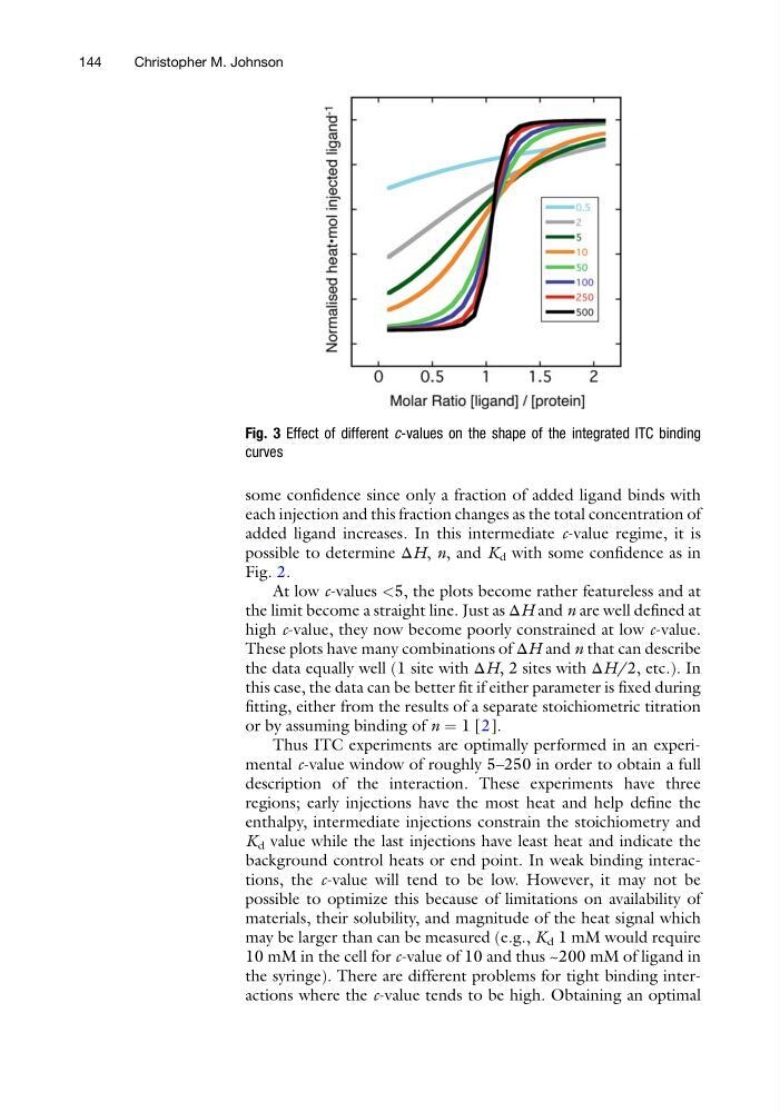
At low c-values <5, the plots become rather featureless and at
the limit become a straight line. Just as ΔH and n are well defined at
high c-value, they now become poorly constrained at low c-value.
These plots have many combinations of ΔH and n that can describe
the data equally well (1 site with ΔH, 2 sites with ΔH/2, etc.). In
this case, the data can be better fit if either parameter is fixed during
fitting, either from the results of a separate stoichiometric titration
or by assuming binding of n ¼ 1 [2].
Thus ITC experiments are optimally performed in an experimental c-value window of roughly 5–250 in order to obtain a full
description of the interaction. These experiments have three
regions; early injections have the most heat and help define the
enthalpy, intermediate injections constrain the stoichiometry and
K d value while the last injections have least heat and indicate the
background control heats or end point. In weak binding interactions, the c-value will tend to be low. However, it may not be
possible to optimize this because of limitations on availability of
materials, their solubility, and magnitude of the heat signal which
may be larger than can be measured (e.g., K d 1 mM would require
10 mM in the cell for c-value of 10 and thus ~200 mM of ligand in
the syringe). There are different problems for tight binding interactions where the c-value tends to be high. Obtaining an optimal
Fig. 3 Effect of different c-values on the shape of the integrated ITC binding
curves
144
Christopher M. Johnson
each injection and this fraction changes as the total concentration of
added ligand increases. In this intermediate c-value regime, it is
possible to determine ΔH, n, and K d with some confidence as in
Fig. 2.
At low c-values <5, the plots become rather featureless and at
the limit become a straight line. Just as ΔH and n are well defined at
high c-value, they now become poorly constrained at low c-value.
These plots have many combinations of ΔH and n that can describe
the data equally well (1 site with ΔH, 2 sites with ΔH/2, etc.). In
this case, the data can be better fit if either parameter is fixed during
fitting, either from the results of a separate stoichiometric titration
or by assuming binding of n ¼ 1 [2].
Thus ITC experiments are optimally performed in an experimental c-value window of roughly 5–250 in order to obtain a full
description of the interaction. These experiments have three
regions; early injections have the most heat and help define the
enthalpy, intermediate injections constrain the stoichiometry and
K d value while the last injections have least heat and indicate the
background control heats or end point. In weak binding interactions, the c-value will tend to be low. However, it may not be
possible to optimize this because of limitations on availability of
materials, their solubility, and magnitude of the heat signal which
may be larger than can be measured (e.g., K d 1 mM would require
10 mM in the cell for c-value of 10 and thus ~200 mM of ligand in
the syringe). There are different problems for tight binding interactions where the c-value tends to be high. Obtaining an optimal
Fig. 3 Effect of different c-values on the shape of the integrated ITC binding
curves
144
Christopher M. Johnson