

3.2 Dealing
with Second-Order
Conditions
Sometimes experimental conditions may be limited by protein
concentrations, signal amplitudes, and rate constants and must
therefore be performed under second order rather than pseudofirst-order conditions. The analysis is a little more complicated but
there are two approaches for dealing with second-order conditions.
The first is to analyze all binding traces simultaneously using
numerical fitting in free software such as Dynafit (http://www.
biokin.com) [18] or other commercial software such as KinTek
[19] or MATLAB. In such global fitting of experimental traces,
k obs values will not be obtained but the output will be the k on and
k off values, and fits to each experimental transient where residuals
can be analyzed. The second option is to fit individual traces to a
single exponential despite being in the second-order region. If they
fit well to a single exponential, k obs may be plotted versus [B] and
fitted to
k obs ¼
ffiffiffiffiffiffiffiffiffiffiffiffiffiffiffiffiffiffiffiffiffiffiffiffiffiffiffiffiffiffiffiffiffiffiffiffiffiffiffiffiffiffiffiffiffiffiffiffiffiffiffiffiffiffiffiffiffiffiffiffiffiffiffiffiffiffiffiffiffiffiffiffiffiffiffiffiffiffiffiffiffiffiffiffiffiffiffiffiffiffiffiffiffiffiffiffi ffi
k
2
on A
½ 0 À B
½ 0
À
Á 2 þ k
2
off þ 2k on k off A
½ 0 þ B
½ 0
À
Á
q
ð3Þ
where [A] 0 and [B] 0 are the initial concentrations of the respective
proteins. This equation accounts for second-order conditions at
low [B] 0 and approaches a linear function at high [B] 0 as in Eq. 2
under pseudo-first-order conditions [20].
a
b
c
Time (s)
Time (s)
Time (s)
Time (s)
Residuals
Residuals
Residuals
Fluorescence intensity
Fluorescence intensity
Fluorescence intensity
Time (s)
Time (s)
0.00
0.05
0.10
0.15
0.20
-0.04
0.00
0.04
0.00
0.05
0.10
0.15
0.20
2.6
2.7
2.8
2.9
0.00
0.05
0.10
-0.1
0.0
0.1
0.0
0.2
0.4
0.6
-0.2
0.0
0.2
0.00
0.05
0.10
4.6
4.8
5.0
5.2
5.4
0.0
0.2
0.4
0.6
5.2
5.4
5.6
5.8
6.0
6.2
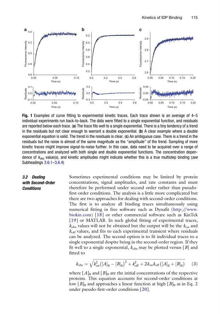
Fig. 1 Examples of curve fitting to experimental kinetic traces. Each trace shown is an average of 4–5
individual experiments run back-to-back. The data were fitted to a single exponential function, and residuals
are reported below each trace. (a) The trace fits well to a single exponential. There is a tiny tendency of a trend
in the residuals but not clear enough to warrant a double exponential. (b) A clear example where a double
exponential equation is valid. The trend in the residuals is clear. (c) An ambiguous case. There is a trend in the
residuals but the noise is almost of the same magnitude as the “amplitude” of the trend. Sampling of more
kinetic traces might improve signal-to-noise further. In this case, data need to be acquired over a range of
concentrations and analyzed with both single and double exponential functions. The concentration dependence of k obs value(s), and kinetic amplitudes might indicate whether this is a true multistep binding (see
Subheadings 3.6.1–3.6.4)
Kinetics of IDP Binding
115
with Second-Order
Conditions
Sometimes experimental conditions may be limited by protein
concentrations, signal amplitudes, and rate constants and must
therefore be performed under second order rather than pseudofirst-order conditions. The analysis is a little more complicated but
there are two approaches for dealing with second-order conditions.
The first is to analyze all binding traces simultaneously using
numerical fitting in free software such as Dynafit (http://www.
biokin.com) [18] or other commercial software such as KinTek
[19] or MATLAB. In such global fitting of experimental traces,
k obs values will not be obtained but the output will be the k on and
k off values, and fits to each experimental transient where residuals
can be analyzed. The second option is to fit individual traces to a
single exponential despite being in the second-order region. If they
fit well to a single exponential, k obs may be plotted versus [B] and
fitted to
k obs ¼
ffiffiffiffiffiffiffiffiffiffiffiffiffiffiffiffiffiffiffiffiffiffiffiffiffiffiffiffiffiffiffiffiffiffiffiffiffiffiffiffiffiffiffiffiffiffiffiffiffiffiffiffiffiffiffiffiffiffiffiffiffiffiffiffiffiffiffiffiffiffiffiffiffiffiffiffiffiffiffiffiffiffiffiffiffiffiffiffiffiffiffiffiffiffiffiffi ffi
k
2
on A
½ 0 À B
½ 0
À
Á 2 þ k
2
off þ 2k on k off A
½ 0 þ B
½ 0
À
Á
q
ð3Þ
where [A] 0 and [B] 0 are the initial concentrations of the respective
proteins. This equation accounts for second-order conditions at
low [B] 0 and approaches a linear function at high [B] 0 as in Eq. 2
under pseudo-first-order conditions [20].
a
b
c
Time (s)
Time (s)
Time (s)
Time (s)
Residuals
Residuals
Residuals
Fluorescence intensity
Fluorescence intensity
Fluorescence intensity
Time (s)
Time (s)
0.00
0.05
0.10
0.15
0.20
-0.04
0.00
0.04
0.00
0.05
0.10
0.15
0.20
2.6
2.7
2.8
2.9
0.00
0.05
0.10
-0.1
0.0
0.1
0.0
0.2
0.4
0.6
-0.2
0.0
0.2
0.00
0.05
0.10
4.6
4.8
5.0
5.2
5.4
0.0
0.2
0.4
0.6
5.2
5.4
5.6
5.8
6.0
6.2
Fig. 1 Examples of curve fitting to experimental kinetic traces. Each trace shown is an average of 4–5
individual experiments run back-to-back. The data were fitted to a single exponential function, and residuals
are reported below each trace. (a) The trace fits well to a single exponential. There is a tiny tendency of a trend
in the residuals but not clear enough to warrant a double exponential. (b) A clear example where a double
exponential equation is valid. The trend in the residuals is clear. (c) An ambiguous case. There is a trend in the
residuals but the noise is almost of the same magnitude as the “amplitude” of the trend. Sampling of more
kinetic traces might improve signal-to-noise further. In this case, data need to be acquired over a range of
concentrations and analyzed with both single and double exponential functions. The concentration dependence of k obs value(s), and kinetic amplitudes might indicate whether this is a true multistep binding (see
Subheadings 3.6.1–3.6.4)
Kinetics of IDP Binding
115