

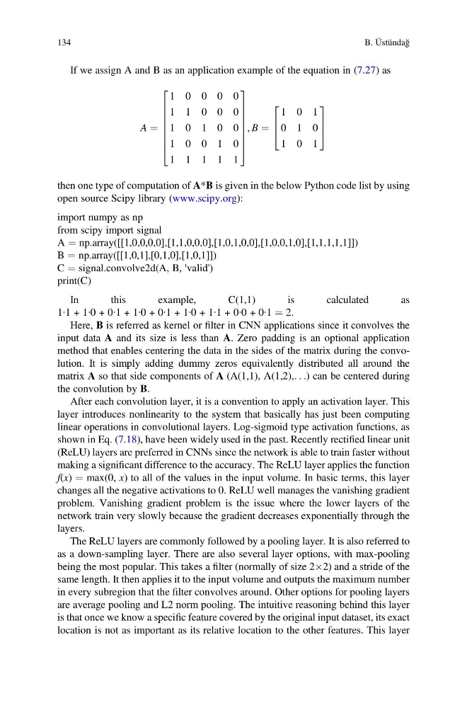
If we assign A and B as an application example of the equation in (7.27) as
A ¼
1 0 0 0 0
1 1 0 0 0
1 0 1 0 0
1 0 0 1 0
1 1 1 1 1
2
6
6
6
6
6
6
4
3
7
7
7
7
7
7
5
, B ¼
1 0 1
0 1 0
1 0 1
2
6
4
3
7
5
then one type of computation of A*B is given in the below Python code list by using
open source Scipy library (www.scipy.org):
import numpy as np
from scipy import signal
A ¼ np.array([[1,0,0,0,0],[1,1,0,0,0],[1,0,1,0,0],[1,0,0,1,0],[1,1,1,1,1]])
B ¼ np.array([[1,0,1],[0,1,0],[1,0,1]])
C ¼ signal.convolve2d(A, B, 'valid')
print(C)
In
this
example,
C(1,1)
is
calculated
as
1∙1 + 1∙0 + 0∙1 + 1∙0 + 0∙1 + 1∙0 + 1∙1 + 0∙0 + 0∙1 ¼ 2.
Here, B is referred as kernel or filter in CNN applications since it convolves the
input data A and its size is less than A. Zero padding is an optional application
method that enables centering the data in the sides of the matrix during the convolution. It is simply adding dummy zeros equivalently distributed all around the
matrix A so that side components of A (A(1,1), A(1,2),. . .) can be centered during
the convolution by B.
After each convolution layer, it is a convention to apply an activation layer. This
layer introduces nonlinearity to the system that basically has just been computing
linear operations in convolutional layers. Log-sigmoid type activation functions, as
shown in Eq. (7.18), have been widely used in the past. Recently rectified linear unit
(ReLU) layers are preferred in CNNs since the network is able to train faster without
making a significant difference to the accuracy. The ReLU layer applies the function
f(x) ¼ max(0, x) to all of the values in the input volume. In basic terms, this layer
changes all the negative activations to 0. ReLU well manages the vanishing gradient
problem. Vanishing gradient problem is the issue where the lower layers of the
network train very slowly because the gradient decreases exponentially through the
layers.
The ReLU layers are commonly followed by a pooling layer. It is also referred to
as a down-sampling layer. There are also several layer options, with max-pooling
being the most popular. This takes a filter (normally of size 2Â2) and a stride of the
same length. It then applies it to the input volume and outputs the maximum number
in every subregion that the filter convolves around. Other options for pooling layers
are average pooling and L2 norm pooling. The intuitive reasoning behind this layer
is that once we know a specific feature covered by the original input dataset, its exact
location is not as important as its relative location to the other features. This layer
134
B. Üstündağ
A ¼
1 0 0 0 0
1 1 0 0 0
1 0 1 0 0
1 0 0 1 0
1 1 1 1 1
2
6
6
6
6
6
6
4
3
7
7
7
7
7
7
5
, B ¼
1 0 1
0 1 0
1 0 1
2
6
4
3
7
5
then one type of computation of A*B is given in the below Python code list by using
open source Scipy library (www.scipy.org):
import numpy as np
from scipy import signal
A ¼ np.array([[1,0,0,0,0],[1,1,0,0,0],[1,0,1,0,0],[1,0,0,1,0],[1,1,1,1,1]])
B ¼ np.array([[1,0,1],[0,1,0],[1,0,1]])
C ¼ signal.convolve2d(A, B, 'valid')
print(C)
In
this
example,
C(1,1)
is
calculated
as
1∙1 + 1∙0 + 0∙1 + 1∙0 + 0∙1 + 1∙0 + 1∙1 + 0∙0 + 0∙1 ¼ 2.
Here, B is referred as kernel or filter in CNN applications since it convolves the
input data A and its size is less than A. Zero padding is an optional application
method that enables centering the data in the sides of the matrix during the convolution. It is simply adding dummy zeros equivalently distributed all around the
matrix A so that side components of A (A(1,1), A(1,2),. . .) can be centered during
the convolution by B.
After each convolution layer, it is a convention to apply an activation layer. This
layer introduces nonlinearity to the system that basically has just been computing
linear operations in convolutional layers. Log-sigmoid type activation functions, as
shown in Eq. (7.18), have been widely used in the past. Recently rectified linear unit
(ReLU) layers are preferred in CNNs since the network is able to train faster without
making a significant difference to the accuracy. The ReLU layer applies the function
f(x) ¼ max(0, x) to all of the values in the input volume. In basic terms, this layer
changes all the negative activations to 0. ReLU well manages the vanishing gradient
problem. Vanishing gradient problem is the issue where the lower layers of the
network train very slowly because the gradient decreases exponentially through the
layers.
The ReLU layers are commonly followed by a pooling layer. It is also referred to
as a down-sampling layer. There are also several layer options, with max-pooling
being the most popular. This takes a filter (normally of size 2Â2) and a stride of the
same length. It then applies it to the input volume and outputs the maximum number
in every subregion that the filter convolves around. Other options for pooling layers
are average pooling and L2 norm pooling. The intuitive reasoning behind this layer
is that once we know a specific feature covered by the original input dataset, its exact
location is not as important as its relative location to the other features. This layer
134
B. Üstündağ