

518 CHAPTER 8. LABORATORY MEASUREMENT AND ANALYSIS
and
Fi = Hi cos(atr) 4- Gi sin(<7tr)
(8.80)
The terms Zi and Y, are given by Eqns. 8.33 and 8.34, respectively.
Equations 8.75 - 8.78 represent a system of four equations with four
unknowns (a^, ür,,
and
for each frequency component. These
unknowns are expressed in terms of the Fourier coefficients (C,-, Dit Gi, and
Hi) that can be determined by fast-Fourier analysis of the two velocity time
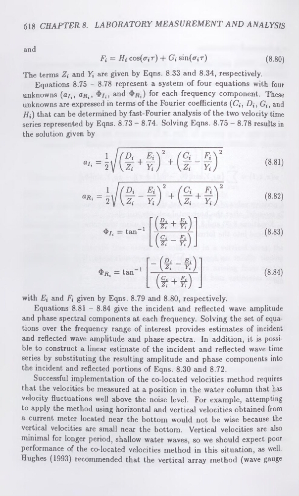
series represented by Eqns. 8.73 - 8.74. Solving Eqns. 8.75 - 8.78 results in
the solution given by
with Ei and Fi given by Eqns. 8.79 and 8.80, respectively.
Equations 8.81 - 8.84 give the incident and reflected wave amplitude
and phase spectral components at each frequency. Solving the set of equations over the frequency range of interest provides estimates of incident
and reflected wave amplitude and phase spectra. In addition, it is possible to construct a linear estimate of the incident and reflected wave time
series by substituting the resulting amplitude and phase components into
the incident and reflected portions of Eqns. 8.30 and 8.72.
Successful implementation of the co-located velocities method requires
that the velocities be measured at a position in the water column that has
velocity fluctuations well above the noise level. For example, attempting
to apply the method using horizontal and vertical velocities obtained from
a current meter located near the bottom would not be wise because the
vertical velocities are small near the bottom. Vertical velocities are also
minimal for longer period, shallow water waves, so we should expect poor
performance of the co-located velocities method in this situation, as well.
Hughes (1993) recommended that the vertical array method (wave gauge
and
Fi = Hi cos(atr) 4- Gi sin(<7tr)
(8.80)
The terms Zi and Y, are given by Eqns. 8.33 and 8.34, respectively.
Equations 8.75 - 8.78 represent a system of four equations with four
unknowns (a^, ür,,
and
for each frequency component. These
unknowns are expressed in terms of the Fourier coefficients (C,-, Dit Gi, and
Hi) that can be determined by fast-Fourier analysis of the two velocity time
series represented by Eqns. 8.73 - 8.74. Solving Eqns. 8.75 - 8.78 results in
the solution given by
with Ei and Fi given by Eqns. 8.79 and 8.80, respectively.
Equations 8.81 - 8.84 give the incident and reflected wave amplitude
and phase spectral components at each frequency. Solving the set of equations over the frequency range of interest provides estimates of incident
and reflected wave amplitude and phase spectra. In addition, it is possible to construct a linear estimate of the incident and reflected wave time
series by substituting the resulting amplitude and phase components into
the incident and reflected portions of Eqns. 8.30 and 8.72.
Successful implementation of the co-located velocities method requires
that the velocities be measured at a position in the water column that has
velocity fluctuations well above the noise level. For example, attempting
to apply the method using horizontal and vertical velocities obtained from
a current meter located near the bottom would not be wise because the
vertical velocities are small near the bottom. Vertical velocities are also
minimal for longer period, shallow water waves, so we should expect poor
performance of the co-located velocities method in this situation, as well.
Hughes (1993) recommended that the vertical array method (wave gauge