

410
CHAPTER 7. LABORATORY WAVE GENERATION
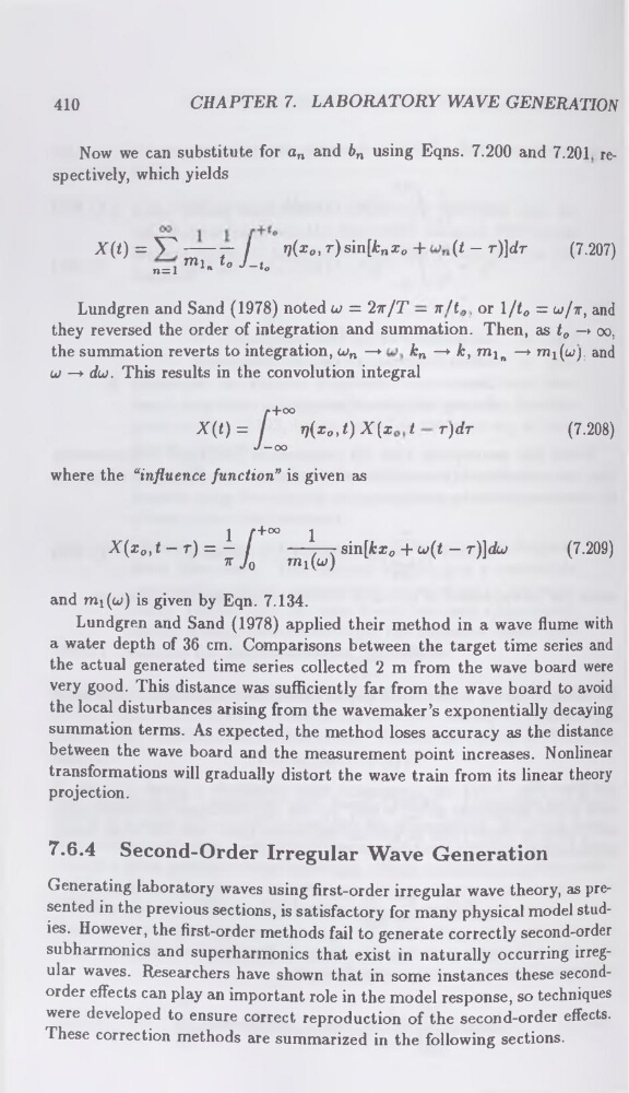
Now we can substitute for an and bn using Eqns. 7.200 and 7.201 respectively, which yields
X(/) = V----- — /
rflxo, r) sin[fcn xo 4(t - r)]dr
n=1 min to J-to
(7.207)
Lundgren and Sand (1978) noted cu = Tn fT — m[Lo, or I/to = u/n, and
they reversed the order of integration and summation. Then, as t0 -> oo,
the summation reverts to integration, u>n —*
kn —* k, mln —► mfu), and
u —+ du). This results in the convolution integral
%(() =
rj(x0,i) X(x t r)dr
(7.208)
where the “influence function” is given as
X(xo,t- r) = 1 /+°° 1
7T Jo
mi(u)
sin[Arx0 + w(/ — r)]cL>
(7.209)
and nii(w) is given by Eqn. 7.134.
Lundgren and Sand (1978) applied their method in a wave flume with
a water depth of 36 cm. Comparisons between the target time series and
the actual generated time series collected 2 m from the wave board were
very good. This distance was sufficiently far from the wave board to avoid
the local disturbances arising from the wavemaker’s exponentially decaying
summation terms. As expected, the method loses accuracy as the distance
between the wave board and the measurement point increases. Nonlinear
transformations will gradually distort the wave train from its linear theory
projection.
7.6.4 Second-Order Irregular Wave Generation
Generating laboratory waves using first-order irregular wave theory, as presented in the previous sections, is satisfactory for many physical model studies. However, the first-order methods fail to generate correctly second-order
subharmonics and superharmonics that exist in naturally occurring irregular waves. Researchers have shown that in some instances these secondorder effects can play an important role in the model response, so techniques
were developed to ensure correct reproduction of the second-order effects.
These correction methods are summarized in the following sections.
CHAPTER 7. LABORATORY WAVE GENERATION
Now we can substitute for an and bn using Eqns. 7.200 and 7.201 respectively, which yields
X(/) = V----- — /
rflxo, r) sin[fcn xo 4(t - r)]dr
n=1 min to J-to
(7.207)
Lundgren and Sand (1978) noted cu = Tn fT — m[Lo, or I/to = u/n, and
they reversed the order of integration and summation. Then, as t0 -> oo,
the summation reverts to integration, u>n —*
kn —* k, mln —► mfu), and
u —+ du). This results in the convolution integral
%(() =
rj(x0,i) X(x t r)dr
(7.208)
where the “influence function” is given as
X(xo,t- r) = 1 /+°° 1
7T Jo
mi(u)
sin[Arx0 + w(/ — r)]cL>
(7.209)
and nii(w) is given by Eqn. 7.134.
Lundgren and Sand (1978) applied their method in a wave flume with
a water depth of 36 cm. Comparisons between the target time series and
the actual generated time series collected 2 m from the wave board were
very good. This distance was sufficiently far from the wave board to avoid
the local disturbances arising from the wavemaker’s exponentially decaying
summation terms. As expected, the method loses accuracy as the distance
between the wave board and the measurement point increases. Nonlinear
transformations will gradually distort the wave train from its linear theory
projection.
7.6.4 Second-Order Irregular Wave Generation
Generating laboratory waves using first-order irregular wave theory, as presented in the previous sections, is satisfactory for many physical model studies. However, the first-order methods fail to generate correctly second-order
subharmonics and superharmonics that exist in naturally occurring irregular waves. Researchers have shown that in some instances these secondorder effects can play an important role in the model response, so techniques
were developed to ensure correct reproduction of the second-order effects.
These correction methods are summarized in the following sections.