

4.2. SHORT-WAVE HYDRODYNAMIC MODELS
105
Example 4.1. Wave Transmission in Short-Wave Models
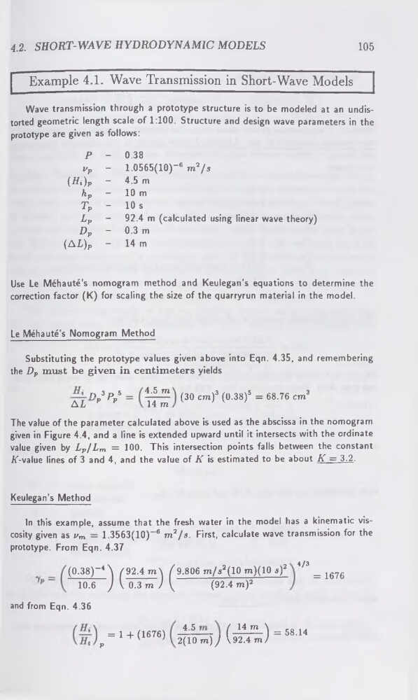
Wave transmission through a prototype structure is to be modeled at an undistorted geometric length scale of 1:100. Structure and design wave parameters in the
prototype are given as follows:
p — 0.38
Up
-
1.0565(10)-® m2 / s
(tf.)p
-
4.5 m
/lp
—
10 m
TP
-
10 s
Lp
-
92.4 m (calculated using linear wave theory)
DP
—
0.3 m
(AL)P
-
14 m
In this example, assume that the fresh water in the model has a kinematic viscosity given as vm — 1.3563(10)“6 m2/s. First, calculate wave transmission for the
prototype. From Eqn. 4.37
4/3
= 1676
and from Eqn. 4.36
4 5
( 14 m. K 58.14
2(10 m) ) \92.4 mJ
Use Le Méhauté’s nomogram method and Keulegan's equations to determine the
correction factor (K) for scaling the size of the quarryrun material in the model.
Le Méhauté’s Nomogram Method
Substituting the prototype values given above into Eqn. 4.35, and remembering
the Dp must be given in centimeters yields
n 3 4 p 5
AL p p
4.5 m
14 m
(30 cm)3 (0.38)5 = 68.76 cm3
The value of the parameter calculated above is used as the abscissa in the nomogram
given in Figure 4.4, and a line is extended upward until it intersects with the ordinate
value given by Lp/Lm = 100. This intersection points falls between the constant
lf-value lines of 3 and 4, and the value of K is estimated to be about K = 3.2.
Keulegan's Method
9.806 m/s2(10 m)(10 a)2
(92.4 m)2
= 1 + (1676)
p
105
Example 4.1. Wave Transmission in Short-Wave Models
Wave transmission through a prototype structure is to be modeled at an undistorted geometric length scale of 1:100. Structure and design wave parameters in the
prototype are given as follows:
p — 0.38
Up
-
1.0565(10)-® m2 / s
(tf.)p
-
4.5 m
/lp
—
10 m
TP
-
10 s
Lp
-
92.4 m (calculated using linear wave theory)
DP
—
0.3 m
(AL)P
-
14 m
In this example, assume that the fresh water in the model has a kinematic viscosity given as vm — 1.3563(10)“6 m2/s. First, calculate wave transmission for the
prototype. From Eqn. 4.37
4/3
= 1676
and from Eqn. 4.36
4 5
( 14 m. K 58.14
2(10 m) ) \92.4 mJ
Use Le Méhauté’s nomogram method and Keulegan's equations to determine the
correction factor (K) for scaling the size of the quarryrun material in the model.
Le Méhauté’s Nomogram Method
Substituting the prototype values given above into Eqn. 4.35, and remembering
the Dp must be given in centimeters yields
n 3 4 p 5
AL p p
4.5 m
14 m
(30 cm)3 (0.38)5 = 68.76 cm3
The value of the parameter calculated above is used as the abscissa in the nomogram
given in Figure 4.4, and a line is extended upward until it intersects with the ordinate
value given by Lp/Lm = 100. This intersection points falls between the constant
lf-value lines of 3 and 4, and the value of K is estimated to be about K = 3.2.
Keulegan's Method
9.806 m/s2(10 m)(10 a)2
(92.4 m)2
= 1 + (1676)
p