Common partial differential equations of computational hydraulics 53
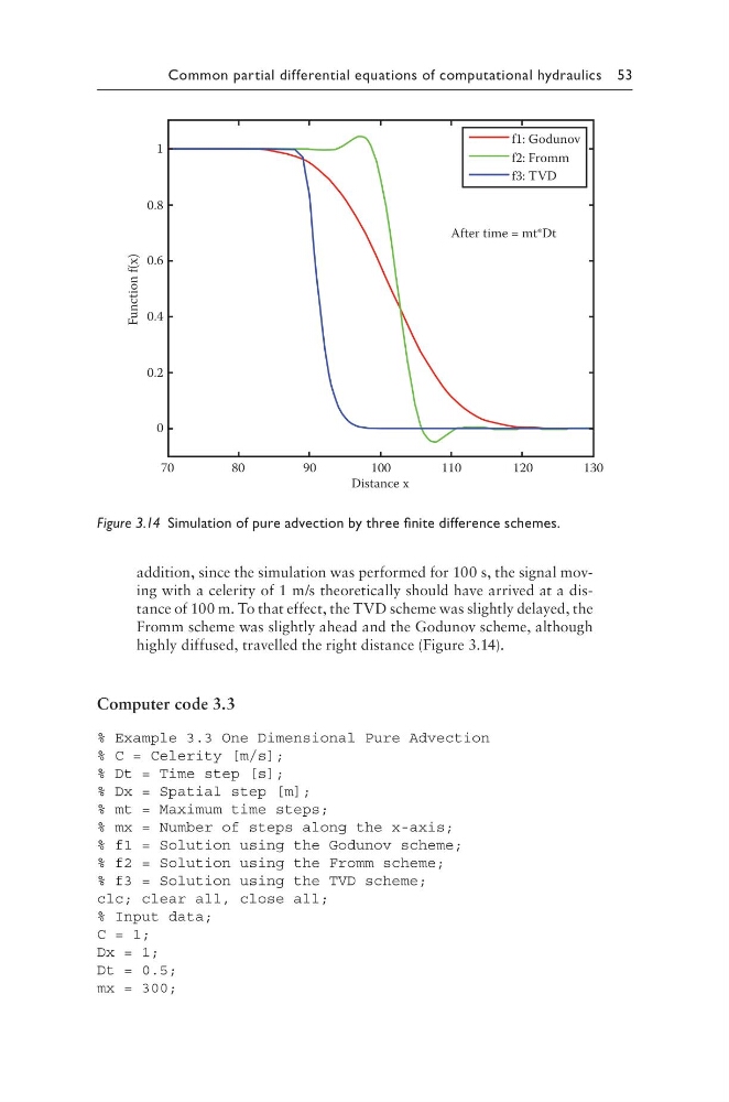
addition, since the simulation was performed for 100 s, the signal moving with a celerity of 1 m/s theoretically should have arrived at a distance of 100 m. To that effect, the TVD scheme was slightly delayed, the
Fromm scheme was slightly ahead and the Godunov scheme, although
highly diffused, travelled the right distance (Figure 3.14).
Computer code 3.3
% Example 3.3 One Dimensional Pure Advection
% C = Celerity [m/s];
% Dt = Time step [s];
% Dx = Spatial step [m];
% mt = Maximum time steps;
% mx = Number of steps along the x-axis;
% f1 = Solution using the Godunov scheme;
% f2 = Solution using the Fromm scheme;
% f3 = Solution using the TVD scheme;
clc; clear all, close all;
% Input data;
C = 1;
Dx = 1;
Dt = 0.5;
mx = 300;
1
0.8
0.6
0.4
0.2
0
70
80
90
100
1 10
120
1 30
Distance x
Function f(x)
After time = mt*Dt
f1: Godunov
f2: Fromm
f3: TVD
Figure 3.14 Simulation of pure advection by three finite difference schemes.