Common partial differential equations of computational hydraulics 51
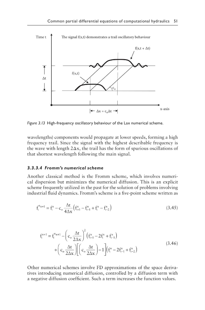
wavelengths) components would propagate at lower speeds, forming a high
frequency trail. Since the signal with the highest describable frequency is
the wave with length 2Δx, the trail has the form of spurious oscillations of
that shortest wavelength following the main signal.
3.3.3.4 Fromm’s numerical scheme
Another classical method is the Fromm scheme, which involves numerical dispersion but minimizes the numerical diffusion. This is an explicit
scheme frequently utilized in the past for the solution of problems involving
industrial fluid dynamics. Fromm’s scheme is a five-point scheme written as
f
f
c
t
x
f
f
f
f
i
n
i
n
o
i
n
i
n
i
n
i
n
* +
+
−
−
= −
−
+ −
(
)
1
1
1
2
4
∆
∆
(3.45)
f
f
c
t
x
f
f f
c
i
n
i
n
o
i
n
i
n
i
n
+
+
+
−
=
−

 

 
−
+
(
)
+
1
1
2
1
1
2
2
*
∆
∆
o o
o
i
n
i
n
i
t
x
c
t
x
f
f
f
∆
∆
∆
∆
2
2
1
2 1

 

 

 

  −






−
+
−
− −
(
)
2
n
(3.46)
Other numerical schemes involve FD approximations of the space derivatives introducing numerical diffusion, controlled by a diffusion term with
a negative diffusion coefficient. Such a term increases the function values.
Δt
Time t
x-axis
f(x,t)
c o
f(x,t + Δt)
Δx = c o Δt
e signal f(x,t) demonstrates a trail oscillatory behaviour
Figure 3.13 High-frequency oscillatory behaviour of the Lax numerical scheme.