

Common partial differential equations of computational hydraulics 49
The implicit and unnoticed introduction, through the selected consistent FD
scheme, of a diffusion term may suppress the anticipated numerical instability, but the effect is so dominant that it causes a diffusion of the f(x,t) values not compatible with the analytical solution of the hyperbolic equation.
Notably, this numerical solution scheme, although inaccurate, is stable and
viable. Also, it can be proven that the numerical scheme is subject to the CFL
stability criterion (Equation 3.29). When the term c
t
x
o
∆
∆
takes its limiting
value (= 1), then the numerical solution is stable and coincides with the analytical solution (the numerical diffusion disappears).
The qualitative reasoning on the stability/instability of the numerical
solution of the first-order hyperbolic equations presented in Equation 3.33
FTCS and Equation 3.36 FTBS can be documented mathematically by
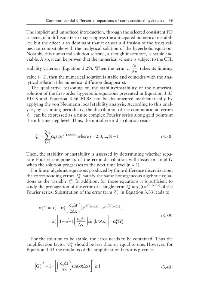
applying the von Neumann local stability analysis. According to this analysis, by assuming periodicity, the distribution of the computational errors
ξ j
n can be expressed as a finite complex Fourier series along grid points at
the nth time step level. Thus, the initial error distribution reads
ξ
α
π
i
k
k x
k
N
t e
where i
N
0
1
1
2
2 3
1
=
=
−
−
=
−
∑ ( )
, ,...,
(
)
∆
(3.38)
Then, the stability or instability is assessed by determining whether separate Fourier components of the error distribution will decay or amplify
when the solution progresses to the next time level (n + 1).
For linear algebraic equations produced by finite difference discretization,
the corresponding errors ξ i
n
satisfy the same homogeneous algebraic equations as the variable f i
n
. In addition, for those equations it is sufficient to
study the propagation of the error of a single term ξ
α
π
k
n
k
k x
t e
=
−
( )
(
)
1 ∆
of the
Fourier series. Substitution of the error term ξ k
n in Equation 3.33 leads to
α
α α
π
π
k
n
k
n
k
n
o
k x
k x
c t
x
e
e
+
−
− −
=
−
−
1
1
1
2
∆
∆
∆
∆
(
)
(
)
=
− −
=
α
π
α
k
n
o
k
n
k
n
c t
x
k x
G
1
1
∆
∆
∆
sin(
)
(3.39)
For the solution to be stable, the error needs to be contained. Thus the
amplification factor G k
n
should be less than or equal to one. However, for
Equation 3.33 the modulus of the amplification factor is given as
G
c t
x
k x
k
n
o
2
2
1
1
= +
≥
∆
∆
∆
sin(
)
π
(3.40)
The implicit and unnoticed introduction, through the selected consistent FD
scheme, of a diffusion term may suppress the anticipated numerical instability, but the effect is so dominant that it causes a diffusion of the f(x,t) values not compatible with the analytical solution of the hyperbolic equation.
Notably, this numerical solution scheme, although inaccurate, is stable and
viable. Also, it can be proven that the numerical scheme is subject to the CFL
stability criterion (Equation 3.29). When the term c
t
x
o
∆
∆
takes its limiting
value (= 1), then the numerical solution is stable and coincides with the analytical solution (the numerical diffusion disappears).
The qualitative reasoning on the stability/instability of the numerical
solution of the first-order hyperbolic equations presented in Equation 3.33
FTCS and Equation 3.36 FTBS can be documented mathematically by
applying the von Neumann local stability analysis. According to this analysis, by assuming periodicity, the distribution of the computational errors
ξ j
n can be expressed as a finite complex Fourier series along grid points at
the nth time step level. Thus, the initial error distribution reads
ξ
α
π
i
k
k x
k
N
t e
where i
N
0
1
1
2
2 3
1
=
=
−
−
=
−
∑ ( )
, ,...,
(
)
∆
(3.38)
Then, the stability or instability is assessed by determining whether separate Fourier components of the error distribution will decay or amplify
when the solution progresses to the next time level (n + 1).
For linear algebraic equations produced by finite difference discretization,
the corresponding errors ξ i
n
satisfy the same homogeneous algebraic equations as the variable f i
n
. In addition, for those equations it is sufficient to
study the propagation of the error of a single term ξ
α
π
k
n
k
k x
t e
=
−
( )
(
)
1 ∆
of the
Fourier series. Substitution of the error term ξ k
n in Equation 3.33 leads to
α
α α
π
π
k
n
k
n
k
n
o
k x
k x
c t
x
e
e
+
−
− −
=
−
−
1
1
1
2
∆
∆
∆
∆
(
)
(
)
=
− −
=
α
π
α
k
n
o
k
n
k
n
c t
x
k x
G
1
1
∆
∆
∆
sin(
)
(3.39)
For the solution to be stable, the error needs to be contained. Thus the
amplification factor G k
n
should be less than or equal to one. However, for
Equation 3.33 the modulus of the amplification factor is given as
G
c t
x
k x
k
n
o
2
2
1
1
= +
≥
∆
∆
∆
sin(
)
π
(3.40)